This is the ground breaking paper by Richard P. Feynman: 'Space-Time Approach to Quantum Electrodynamics'
To be honest, I can read such a paper as if it is a novel, written in French.
Now I cannot really speak French, but I can at least understand a bit of what
they are saying, if they are prepared to pronounce slowly. And that turns out
to be difficult: "Lentement, s'il vous plait, très lentement."
Well, everybody has his specialism. And Quantum ElectroDynamics (QED)
certainly is not mine. Why then this attempt to nevertheless say some
sensible things about it? To our great relief, the following sentence
appears in Feynman's paper, quote from chapter 5:
We desire to make a modification of quantum electrodynamics analogous to
the modification of classical [OK !] electrodynamics described in a previous
article, A. There the δ(s122) appearing in the
action of interaction was replaced by f(s122) where f(x)
is a function of small width and great height.
Further support of this idea is found in the very well readable
Richard P. Feynman - Nobel Lecture :
There were several suggestions for interesting modifications of electrodynamics. We discussed lots of them, but I shall report on only one. It was to replace this delta function in the interaction by another function, say, f(I2ij), which is not infinitely sharp. Instead of having the action occur only when the interval between the two charges is exactly zero, we would replace the delta function of I2 by a narrow peaked thing. Let's say that f(Z) is large only near Z=0 width of order a2. Interactions will now occur when T2-R2 is of order a2 roughly where T is the time difference and R is the separation of the charges. This might look like it disagrees with experience, but if a is some small distance, like 10-13 cm, it says that the time delay T in action is roughly √ (R2 ± a2) or approximately, - if R is much larger than a, T = R ± a2/2R. This means that the deviation of time T from the ideal theoretical time R of Maxwell, gets smaller and smaller, the further the pieces are apart. Therefore, all theories involving in analyzing generators, motors, etc., in fact, all of the tests of electrodynamics that were available in Maxwell's time, would be adequately satisfied if were 10-13 cm. If R is of the order of a centimeter this deviation in T is only 10-26 parts. So, it was possible, also, to change the theory in a simple manner and to still agree with all observations of classical electrodynamics. You have no clue of precisely what function to put in for f, but it was an interesting possibility to keep in mind when developing quantum electrodynamics.
It is noted that much of this classical
electrodynamics theory is also found in 'The Feynman Lectures on Physics'
Part II, chapter 28: 'Electromagnetic mass'. In paragraph 28-5, which is titled
'Attempts to modify the Maxwell theory' we read (at page 28-8) about 'another
modification of the laws of electrodynamics as proposed by Bopp'. Bopp's theory
is that: Aμ(1,t1) = ∫
jμ(2,t2) F(s122)
dV2 dt2
It's important to observe that the above integral has all characteristics
of a convolution integral with F as a kernel.You may forget all
the rest, but remember this !
Subsequent quotes are aimed at showing that Feynman actually did copy the
method "with δ replaced by a function of small width and great height",
from classical electrodynamics to quantum electrodynamics:
Anyway, it forced me to go back over all this and to convince myself physically
that nothing can go wrong. At any rate, the correction to mass was now finite,
proportional to ln(m.a/h) (where a is the width of that function f which was
substituted
for δ). If you wanted an unmodified electrodynamics, you would have to
take a equal to zero, getting an infinite mass correction. But, that wasn't the
point. Keeping a finite, I simply followed the program outlined by Professor
Bethe and showed how to calculate all the various things, the scatterings of
electrons from atoms without radiation, the shifts of levels and so forth,
calculating everything in terms of the experimental mass, and noting that the
results as Bethe suggested, were not sensitive to a in this form and even had
a definite limit as a → 0.
[ ... snip ... ]
It must be clearly understood that in all this work, I was representing the
conventional electrodynamics with retarded interaction, and not my halfadvanced
and half-retarded theory corresponding to (1). I merely use (1) to guess at
forms. And, one of the forms I guessed at corresponded to changing δ to
a function f of width a2, so that I could calculate finite results
for all of the problems. This brings me to the second thing that was missing
when I published the paper, an unresolved difficulty. With δ replaced by
f the calculations would give results which were not "unitary", that is, for
which the sum of the probabilities of all alternatives was not unity. The
deviation from unity was very small, in practice, if a was very small. In the
limit that I took a very tiny, it might not make any difference. And, so the
process of the renormalization could be made, you could calculate everything in
terms of the experimental mass and then take the limit and the apparent
difficulty that the unitary is violated temporarily seems to disappear.
I was unable to demonstrate that, as a matter of fact, it does.
That was in 1965. Since then, a zillion proposals have been done to get rid of the "infinities" in Quantum Electrodynamics. Shall we summarize the situation?
But, some people seemingly succeed in keeping sort of order in the chaos. People such as John Baez. He has written many lucid articles on Mathematical Physics, this one for example:
Renormalization Made Easy (but where is it?)
We are talking here about the "oldest game", which is Feynman's game. A rather new development is the approach via "renormalization groups" by Kenneth Wilson (1982). Giving rise, again, to an interesting quote:
Wilson's analysis takes just the opposite point of view, that any quantum field theory is defined fundamentally with a distance cutoff D that has some physical significance. In statistical mechanical applications, this distance scale is the atomic spacing. In quantum electrodynamics and other quantum field theories appropriate to elementary particle physics, the cutoff would have to be associated with some fundamental graininess of spacetime, [ ... snip ... ] But whatever this scale is, it lies far beyond the reach of present-day experiments. Wilson's arguments show that this this circumstance explains the renormalizability of quantum electrodynamics and other quantum field theories of particle interactions. [ ... snip ... ]
There is also a popularized version of Quantum ElectroDynamics theory:
Feynman's book
'QED: The Strange Theory of Light and Matter'.
The effects of Gaussian broadening may be visualized
as follows.
Work in Progress
Time to come to a summary. We find that the "oldest renormalization game" is
actually nothing else than the following. Point-like interaction, as formalized
by the presence of a delta-function in sort of a convolution integral, is being
replaced by interaction over a short distance, as formalized by the presence of
a "function f of small width and great height" in the same convolution integral.
The "width" of that function f is the infamous "cut-off" value in QED. Hence we
must work the other way around. Instead of considering a delta function as the
sharp (desirable) limiting shape of i.e. a Gaussian distribution, we must now
consider (for example) a Gauss distribution as the (desirable) broadening
of a delta function. Both kind of functions occur as the kernels in convolution
integrals. Where have we seen all of this before? When formulated in this way,
the situation in Quantum ElectroDynamics is by no way unique. You really don't
need elementary particles for being able to do fundamental research.
For the sake of clarity, any "function of small width and great height", which
converges to a delta-function as the width → 0, will be called a shape
function in the sequel. To be more precise: it's a shape function in the
sense of a Finite Volume Method. There is no confusion, actually, because the
shape functions in Numerical Analysis are a subclass of the shape functions in
our Fuzzy Analysis.
(This work is not perfect yet. Improvements have been suggested by Robert Low,
as seen in a subtread of 'Probability in an infinite sample space' (sci.math):
1 , 2 , 3 , 4 , 5 .
In the same document, a result is established
which is quite relevant here: Gaussian Smoothing is represented by an operator
exp( 1/2 σ2 d/dx2 )
But the theory of Fuzzyfied Logic, which is contained in the same
documentation &
software bundle, is even more appropriate for this application.
Here is a visualization of the fuzzyfied equality, as a
function of x and y, according to the latter theory.
The Top Down Approach
The Discrete finds its origin in Mathematics itself. Originally, it has been
associated with the art of
counting. Not so with the Continuum. The continuum finds its origin in
measurements, especially in Geometry, hence in Physics. There is some truth
in Newton's remark "for the description of right lines and circles, upon
which geometry is founded, belongs to mechanics", as quoted from: Preface
to Isaac Newton's
Principia (1687). Pure mechanics is thus really very close to pure
mathematics: kinematics = geometry + time , dynamics = kinematics + mass .
Anyway, the continuum has as its main characteristic that it is not countable,
but measurable (in a physical sense).
We can conclude that the Discrete is Bottom-Up (accessible through counting)
while the Continuous is Top-Down (accessible through measuring). We can see,
however, that some top-down techniques can also be associated with discrete
things, like paying with Euro's. The reverse is
also true: the continuum can be discretized and hence made accessible
through counting (maybe accounting: bookkeeping). That's what Numerical
Analysis is all about. It turns out that the problem of the Continuum,
there, is not so much in continuity as such, but merely in its relationship to
the Discrete.
As opposed to Discretization, how about Continuization ? What if not only top-down methods can be employed with the discrete, but even the discrete itself can be made continuous ? In fact, this is what actually happens with our Numerical Methods, as soon as discrete points are associated with so-called Shape Functions, in order to enable differentiation and integration. The latter being actions which are typically in the need of a continuous (and even analytical) domain. Finite element shape functions (or rather interpolations) are among the most elementary examples of functions which can be employed for the purpose of making a discrete substrate continuous (again). But there are others, like the bell shaped Gaussian curves, employed with Fuzzy Analysis. We have already decided to use the same name for these and for the shape functions in Numerical Analysis as well. I think what Applied needs is no more discretization, but continuization instead ;-)
An interesting pattern is emerging now. It is known that a continuous function can be discretized (sampled) by convoluting it with a comb of delta-functions. (Examples are in 'Discrete Linear System Summary' & 'Aliasing, Image Sampling and Reconstruction') But we have also seen the reverse now: a discrete function can be made continuous by convoluting it with a comb of shape functions. This is commonly called 'interpolation'. However, if Gaussian distribution functions are being employed as interpolants, then the discrete function values are actually a bit different from the continuized function values at the same place. Summarizing:
Our top down approach may also be called AfterMath :-).
It's After the Mathematics. Post-processing instead of pre-processing.
The taste of the pudding is in the eating. The crucial question is: whether
(renormalization = continuization = Gaussian broadening) according to this
author (HdB) is indeed capable of removing singularities. Due to the
limitations of HTML, two PDF documents have been produced on this issue:
The sources of the first document and (Delphi Pascal) test programs are
included as well. Here are some results, for the
2-D and for the 3-D case
respectively.
A typical example is the ideal gas law: p = c.T/V , where p = pressure,
V = volume, c = constant, at a constant temperature T. No matter how you try,
it's impossible to renormalize the function p(V) for V → 0 . This
is due to the one-dimensional character of it. But, as everybody knows,
nature has found a solution for the zero Volume problem: the ideal gas law is
changed into something else, another law of nature. The gas becomes a
fluid. And, under even more pressure, the fluid becomes a solid.
But, uhm .. on retrospect, it seems that my approach has been more difficult
than necessary. A function 1/r in 2-D
may be simply renormalized
as 1/√(r2 + σ2) and a function
1/r2 in 3-D
may be simply renormalized as
1/(r2 + σ2) : a Cauchy distribution
for the latter. The smaller σ is, the "better". Green lines in the
pictures.
Three additional publications:
But other name calling comes into mind as well. Smoothening can be considered
as the modelling of a measurement process. The mathematical phenomenon is
"sensed", so to speak, with a physical device, a sensor. Sensors always
come with a spread σ , kind of a limited aperture, sort of fuzzyness,
which makes any measurement vulnerable to a certain uncertainty. The common
philosophy still is that these errors are not part of nature itself, but only
part of our methods of observing it. But, according to
Quantum Mechanics, "our" observations are part of the
observed phenomenon itself ! Worse, it's not "us" who are observing nature.
Nature is observing itself, with "us" as a medium, eventually. But not
necessarily. It's no miracle that the electron observes it's own self energy
(the name says it) by sending virtual photons back and forth to itself. It
has a built-in sensor. Thus the sensor, the smoothening kernel, is part of
the physical modelling, even in theory. It may be universal, so let's call it
the Cosmic Sensor eventually. (Not to be confused with "Cosmic Censor" in
the Cosmic
Censorship hypothesis.)
Renormalization of
Singularities
The core activity of renormalization is the calculation of a convolution
integral with a shape function as a kernel. But, with the evaluation of these
integrals, it makes a huge difference whether you integrate in one (dx),
two (dx.dy) or three (dx.dy.dz) dimensions. So the dimensionality (1,2,3,4,..)
is crucial with the successful continuization - yes or no - of singularities.
This argument is, however, misleading. Simplified renormalizations
can only be substituted iff it has been firmly established that the
original functions indeed get lost of their singularities with (the model of)
some measurement. That is: the convolution with a shape function always comes
first, simplification may come afterwards.
Fluid Tube Continuum
One of the most striking examples of Continuization has been the discovery of
the so-called Fluid-Tube Continuum. Well, it's been a long story. At that time,
an international (European) consortium was working on the infamous fast breeder
nuclear reactor in
Kalkar (West Germany).
The Dutch partner in this consortium was called
Neratoom. As an
employee of Neratoom, I have mainly been working on both
sodium
pumps
and the
IHX
(intermediate heat exchanger). It was the
Numerical Analysis of the latter apparatus that has led us to the
Fluid Tube Continuum.
The idea behind this comes from the classical theory of Porous Media.
It is virtually impossible, namely, to apply the original Navier-Stokes / Heat
Transfer equations, together with their boundary conditions, to a truly
detailed model of the tube bundle. With help of the porous media theory,
though, it can be argued that the flow field, as a first approximation, is
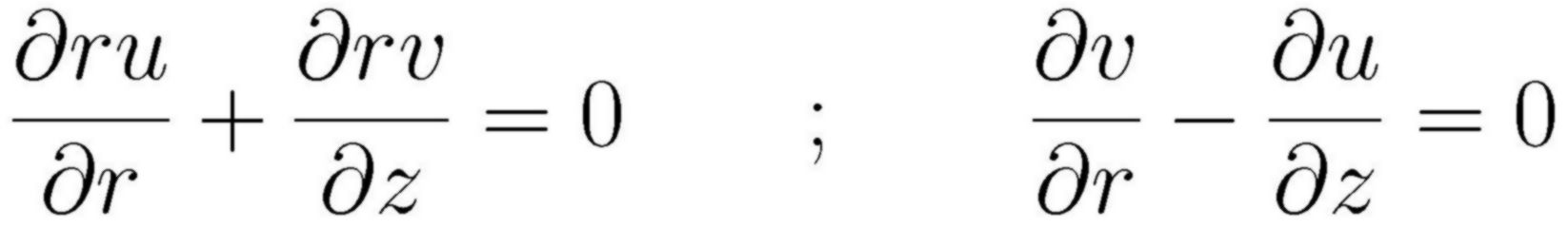
irrotational. Furthermore, the liquid (sodium) is incompressible and it
is contained in a cylinder symmetrical geometry. Such an example of Ideal
Flow is described by the following system of first order PDE's (Partial
Differential Equations):
|
|
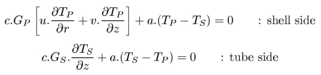
These PDE's have been solved numerically. To that end, the same discretization method as with another ideal flow problem (Labrujère's Problem) has been employed. With help of the fluid tube continuum model, as a next step, the partial differential equations for the primary and secondary temperatures (heat balances) are set up:
|
Having calculated the flow field, the PDE's for the temperature fields have to be solved too. To that end, several methods - none of them very revolutionary - have been employed. The resulting computer program, which calculates both the flow and the temperature fields and compares the latter with real experiments, is in the public domain. Further interesting details are found in a SUNA publication. Especially the statement that the assumption of Ideal Flow also gives rise to a higher safety margin with respect to the temperature stresses deserves attention. A neater representation of the proof hereof is disclosed too.
But the most interesting is that quite unexpected things may happen at the
boundary between the Continuous and the Discrete! BTW, a Dutch version
of the previous has been available for a couple of years ( > 1995); it's
section 6.7 in my book. The
Fluid Tube Continuum has as a tremendous advantage that the granularity
of its discrete substrate is known: it is the pitch of the tube bundle.
It is shown in the
paper
how this continuum breaks down for a certain critical primary mass flow,
which so large, namely, that the heat can no longer be transferred within the
distance of a pitch.
What relationship does there exist between a fluid tube continuum and the
Prime Number Theorem ? Well, according to the prime number theorem,
the (approximate) density of the prime numbers in the neighbourhood of a number
x goes like 1/ln(x) . But, in order to be able to speak of a density,
prime numbers must be subject to, yes: continuization. Like with the
tube bundle of a heat exchanger, discrete items (tubes / primes) must be
blurred, in such a way that things are not visible anymore as separate
objects. In order to accomplish this, the same technology as with numerical differentiation might be employed:
P(x) = Σk fk
e-[(x - xk) / σk]2 / 2
with discrete values fk
at positions xk
σk = √ xk . ln( xk )
(according to an estimate by von Koch)
Indeed, with these spreads, it turns out that the density distribution P(x)
of the prime numbers is approximated very well by the theoretical result:
1/ ln(x) .
Prime Number Theory
Here the spread σ, too, has been made dependent on k . Now make all
function values fk equal to 1 . And next identify the positions
xk with the prime number positions. Then only the following
question remains. What values must be designated to the spreads
σk , in order to accomplish that the series P(x) represents
a (n almost) continuous function ? Don't expect my contributions to
Prime Number Theory to be of the same level as those to Numerical Analysis (?)
But, nevertheless, I want to coin up my 5 cents worth, being the following
conjecture:
According to R.C. Vaughan (February 1990): It is evident that
the primes are randomly distributed but, unfortunately, we don't know what
'random' means.
This is Experiment number 4 in the accompanying software,
where the primes are
replaced by random hits in a Monte Carlo experiment. And very well indeed, the
abovementioned spread σk does not seem to be typical
for prime numbers only !