Latest revision 27-01-2024

index $ \def \hieruit {\quad \Longrightarrow \quad} \def \met {\quad \mbox{with} \quad} \def \EN {\quad \mbox{and} \quad} \def \SP {\quad ; \quad} \def \half {\frac{1}{2}} $

Simplification

In both the Fred Hoyle version and the Halton Arp version of Narlikar's theories it is claimed that the mass of a particle may not stay constant. Two alternative viewpoints are presented to explain how large redshifts could arise from emission of radiation by particles of low masses. Needless to say that we adhere to the alternative viewpoint as exposed in the Narlikar-Arp article. And we find it sort of suspect that a complicated mathematical machinery like the one of General Relativity would be necessary for deriving a simple formula like this: $$ \frac{m}{m_0} = \left(\frac{T-A}{T_0-A}\right)^2 $$ Suppose we have two atomic clocks. Clock number (1) starts ticking at time $0$ and remains doing so over an atomic time lapse which is $\Delta \tau$ ticks long. Clock number (2) starts ticking as soon as the time $\Delta \tau$ at clock number (1) has elapsed. And it remains doing so over an atomic time lapse which is $\Delta \tau$ ticks long. Then it is reasonable to assume that we have a relative variation in mass which is equal to the previous one, because there is only a shift in the origin $\,0 \to \Delta \tau\,$. We have to be careful here. A clock tick $\,\Delta t\,$ in atomic time is not exactly the same as an (in)finitesimal progress $\,\Delta \tau\,$ in that time frame. $$ \frac{\Delta t}{\Delta t_0} = \frac{m_0}{m(\Delta \tau)} = \frac{m(\Delta \tau)}{m(2\Delta \tau)} \hieruit \frac{m(2\Delta \tau)}{m_0} = \frac{m(\Delta \tau)}{m_0}\frac{m(\Delta \tau)}{m_0} $$ Perhaps we have a hidden assumption here: the future will be quite like the past. And there are no jumps, no catastrophic events, no singularities in the flow of (atomic) time. This is known as the Uniformity Principle. Continuing in this way: $$ \frac{m_0}{m(\Delta \tau)} = \frac{m(2\Delta \tau)}{m(3\Delta \tau)} \hieruit \frac{m(3\Delta \tau)}{m_0} = \frac{m(2\Delta \tau)}{m_0}\frac{m(\Delta \tau)}{m_0} = \left[\frac{m(\Delta \tau)}{m_0}\right]^3 $$ And finally: $$ \frac{m(N\Delta \tau)}{m_0} = \left[\frac{m(\Delta \tau)}{m_0}\right]^N $$ For large $N$ and small $\Delta \tau$ as a first order approximation, while atomic time $\,t\,$ is coming into play again: $$ \frac{m(\Delta \tau)}{m_0} \approx 1 + \left.\frac{dm/m_0}{dt}\right|_{t=t_0}.\Delta \tau = 1 + k.\frac{t-t_0}{N} $$ where $k$ is a constant. And so, with $\,\Delta \tau \to dt\,$: $$ \lim_{N\to\infty} \frac{m(N.dt)}{m_0} = \frac{m(t)}{m_0} = \lim_{N\to\infty} \left[1 + k.\frac{t-t_0}{N}\right]^N = e^{k(t-t_0)} $$ It is assumed that cosmological redshifts $\,z\,$ are intrinsic, meaning that they are caused by the Varying Particle Mass (VPM). So we have, from Length Contraction: $$ \boxed{ 1+z_i = \frac{\lambda}{\lambda_0} = \frac{m_0}{m} } $$ Where $\lambda$ and $\lambda_0$ are wavelengths of the emitted radiation, corresponding respectively to $m$ and $m_0$. It follows that $$ 1+z_i = e^{-k(t-t_0)} = e^{k(t_0-t)} \met t \lt t_0 \\ 1+z_i \approx 1+k(t_0-t) \SP z_i \approx k(t_0-t) $$ Meaning that our constant $\,k\,$ can be nothing else than the (intrinsic) Hubble constant: $\,k=H_i\,$. Thus we have, according to Hubble Parameter, for a cosmic distance $D$, still assuming intrinsic redshift all over the place: $$ 1+z_i = e^{H_i(t_0-t)} \SP H_i(t_0-t) = \ln(1+z_i) \\ D = c_0(t_0-t) \hieruit D = \ln(1+z_i)c_0/H_i $$ where $c_0=$ lightspeed and $H_i=$ (intrinsic) Hubble constant. Note that time is running backwards: $(t_0-t)$ is positive.
A more or less preliminary version of this posting is found in thread 160 at GitHub.
The mathematics below is meant as another heuristics for the 'TL' formula $\displaystyle d_A = \frac{c}{H_0}\ln(1+z)$ where we agree upon.

Take a look at the picture, depicting a timeline in cosmos back in time. Let (2) be our position on earth, (1) is the position of a far away civilization like ours, (0) is the position of a galaxy observed by observers on both habitable planets. Let $\lambda=$ wavelength of light. Then it is obvious that: $$ \frac{\lambda_1}{\lambda_0} \frac{\lambda_2}{\lambda_1} = \frac{\lambda_2}{\lambda_0} $$ And therefore, by definition of $z_{ab}=(\lambda_b-\lambda_a)/\lambda_a$ : $$ 1+z_{02} = (1+z_{01})(1+z_{12}) $$ It is reasonable to assume that the whole $\Delta t_{02}$ is the sum of the parts $\Delta t_{01}$ and $\Delta t_{12}$ and so $$ 1+z = F(\Delta t) \quad \mbox{where} \quad F(\Delta t_{02}) = F(\Delta t_{01}).F(\Delta t_{12}) = F(\Delta t_{01} + \Delta t_{12}) $$ This makes the function $F$ a special one, because it is seen now that the following property must hold for all $(t,\tau)$. $$ \ln(F(t+\tau)) = \ln(F(t)) + \ln(F(\tau)) $$ We need another preliminary: Additive functions and measure theory. From that reference we infer that $$ \ln(F(t)) = \kappa.t \quad \Longrightarrow \quad F(t) = 1+z = e^{\kappa.t} $$ where $\kappa$ is a constant that has to be determined from physics. Employing $1+z = e^{\kappa.t} \approx 1+\kappa.t$ and Hubble's law $z = - H_0.t = \kappa.t$ for (relatively) small cosmic lightyears we get that $\kappa=-H_0$ . And $d_A = -c.t$ then leads to the conclusion: $$ 1+z = e^{-H_0.t} \quad \Longrightarrow \quad d_A = \frac{c}{H_0}\ln(1+z) $$
Louis Marmet via A Cosmology Group (18 dec. 2022 04:23) writes: Out of the references I have compiled, most models (72 out of 92) that derive the redshift from a physical process give a logarithmic relationship D = (c/Ho) ln(1 + z). On the other hand we have: $$ 1+z_i = \frac{m_0}{m} = e^{-H_i(t-t_0)} \hieruit \large \boxed{ \frac{m}{m_0} = e^{H_i(t-t_0)} } $$ The presence of $m_0$ and $t_0$ ensures that $m=m_0$ for $t=t_0$. A relevant (Astronomy S.E.) reference in this context is: How is the Universe's Expansion Accelerating if the Hubble Constant is Decreasing? In the accepted answer it is read: A simple piece of maths shows you that the Hubble parameter is a Hubble constant only for an exponential expansion of empty space, which is exactly what we found. Furthermore we have, according to Time Dilation, with $T=$ gravitational time: $$ \frac{dT}{dt} = \sqrt{\frac{m}{m_0}} = e^{H_i/2.(t-t_0)} \hieruit T = \int e^{H_i/2.(t-t_0)} dt = \frac{e^{H_i/2.(t-t_0)}}{H_i/2} + C $$ The boundary condition is $\,T=T_0=t=t_0\,$. It follows that $\,T_0=2/H_i+C\,$ and hence $\,C=T_0-2/H_i\,$: $$ T-T_0 = \frac{2}{H_i}\left[e^{H_i/2.(t-t_0)}-1\right] \hieruit 1+\frac{H_i}{2}(T-T_0) = e^{H_i/2.(t-t_0)} = \sqrt{\frac{m}{m_0}} \\ \hieruit \boxed{ \frac{m}{m_0} = \left[1+\frac{H_i}{2}(T-T_0)\right]^2 } $$ Which is the VPM according to Narlikar's Law, as we shall see. It is worth noticing that General Relativity is not needed at all for the derivation.
The varying particle mass becomes zero for an orbital timestamp $\,T=A\,$, giving back the old Narlikar law as well. $$ 1+\frac{H_i}{2}(A-T_0) = 0 \hieruit H_i/2 = 1/(T_0-A) \SP \boxed{ H_i = \frac{2}{T_0-A} }\\ \frac{m}{m_0} = \left[1+\frac{H_i}{2}(T-T_0)\right]^2 = \left[\frac{T_0-A}{T_0-A}+\frac{T-T_0}{T_0-A}\right]^2 = \left(\frac{T-A}{T_0-A}\right)^2 $$ For the Frequency of Orbital clocks a linear sensible density is found:

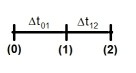
$$ \frac{F}{F_0} = \frac{\Delta T_0}{\Delta T} = \sqrt{\frac{m}{m_0}} = 1+\frac{H_i}{2}(T-T_0) $$ The theory of linear Sensible Densities must be adapted a little bit in order to make physical applications possible (see Dimensions check): $$ P(\tau) = C\tau+D \hieruit \int_{0}^{T_k/\Delta} (C \tau + D ) \, d\tau = \half C \left(\frac{T_k}{\Delta}\right)^2 + D \left(\frac{T_k}{\Delta}\right) = k \\ \frac{T_k}{\Delta} = \sqrt{(D/C)^2 + 2 k/C} - D/C = \sqrt{1/4 + 2 k} - 1/2 = \tau_k \\ \hieruit C=1 \SP D=\frac{1}{2} \SP P(\tau) = \tau + \frac{1}{2} \\ 1+\frac{H_i}{2}(T-T_0) = 2 P\left(\frac{H_i}{4}(T-T_0)\right) $$

It follows that for $(T_0-T)=2/H_i=(T_0-A)$ - near the creation timestamp Alpha - the orbital clock frequency becomes zero. This means that the age $(T_0-A)$ cannot be measured exactly with one of our clocks, neither with an orbital one or with an atomic one.
Let Milne's Formula be the next and the last one to derive. $$ 1+\half H_i (T-T_0) = e^{H_i/2.(t-t_0)} \\ \boxed{ \half H_i(t-t_0) = \ln\left[1+\half H_i (T-T_0)\right] } $$ The old formula can be recovered with $\,(T_0-A) = 2/H_i\,$ or rather $\,\half H_i = 1/(T_0-A)\,$, giving: $$ t-t_0 = (T_0-A)\ln\left[\frac{T_0-A}{T_0-A} + \frac{T-T_0}{T_0-A}\right] = (T_0-A)\ln\left(\frac{T-A}{T_0-A}\right) $$
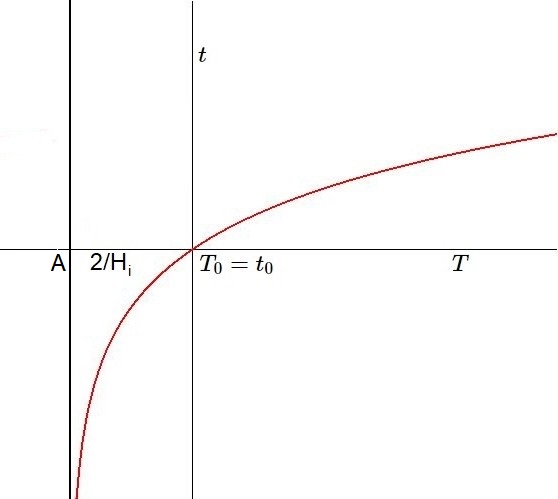