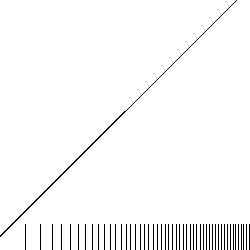
Next consider the case in which the density is increasing in a linear fashion.
What does it mean: linear? Well, suppose there is one point $x_k$ between $0$
and $1$, then there are two points $x_k$ between $1$ and $2$, three points
$x_k$ between $2$ and $3$, and so on. Suppose the initial sampling distance
is $\Delta$. Then, when we arrive at $x = k.\Delta$, the number of points has
been increased to $1+2+3+...+k=k(k+1)/2$. Therefore our basic equation is:
$$
x_{k(k+1)/2} = L.\Delta \qquad \mbox{where:} \quad k,L = 1,2,3, ...
$$
In this way, the array $x$ is only defined for certain values of its index,
namely: $1,3,6, ...$. In order to generalize for all values of the index, $k$
must be solved from:
$$
k(k+1)/2 = L \hieruit k^2+k-2L = 0 \hieruit k = \frac{\sqrt{8 L+1}-1}{2}
$$
It is concluded that a monotone sequence with a linearly increasing density may
be represented by:
$$
x_L = \frac{\sqrt{8 L+1}-1}{2} \Delta \OF
x_k = \left( \sqrt{1/4 + 2 k}-1/2 \right) \Delta
$$
The first few values (for $\Delta = 1$):
$$
x_0 = 0 \: , \: x_1 = 1 \: , \: x_2 = 1.56155 \: , \: x_3 = 2 \: , \:
x_4 = 2.37228 \: , \: x_5 = 2.70156 \: , \: x_6 = 3 \: , \: ...
$$
Other exact densities can be constructed by demanding that the integral
over its sense $P$, from $x_k$ to $x_{k+1}$, is equal to unity:
$$
\int_{x_k}^{x_{k+1}} P(t) \, dt = 1
$$
Simple theorem:
$$
\int_{x_0}^{x_k} P(t) \, dt = k
$$
Proof by complete induction:
\begin{eqnarray*}
&& \int_{x_0}^{x_1} P(t) \, dt = 1 \\
&& \int_{x_0}^{x_k} P(t) \, dt = k \hieruit \\
&& \int_{x_0}^{x_{k+1}} P(t) \, dt =
\int_{x_0}^{x_k} P(t) \, dt + \int_{x_k}^{x_{k+1}} P(t) \, dt = k+1
\end{eqnarray*}
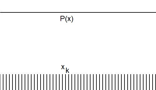
Specify for the constant sense, which is given by $P(x)=1/\Delta$,
where $\Delta$ is a uniform sampling distance:
$$
\int_{x_0}^{x_k} 1/\Delta \, dt = (x_k-x_0)/\Delta = k
\hieruit x_k = x_0 + k.\Delta
$$
Another example is the linear sense, which is given by
$P(x)=C x + D$. It is no restriction on generality if the starting value $x_0$
of $x_k$ is simply put to zero here. Then the integral becomes:
$$
\int_{0}^{x_k} (C t + D ) \, dt = \half C x_k^2 + D x_k = k
\hieruit x_k = \sqrt{(D/C)^2 + 2 k/C} - D/C
$$
But wait! This outcome has to be compared with the one we have obtained in an
earlier stage:
\begin{eqnarray*}
\mbox{Compare} \qquad x_k = \left( \sqrt{1/4 + 2 k}-1/2 \right) \Delta \\
\mbox{with} \qquad x_k = \sqrt{(D/C)^2 + 2 k/C} - D/C
\end{eqnarray*}
A perfect match is found for $D/C = \half\Delta$ and $C = 1/\Delta^2$.
Conclusion:
$$
P(x) = C(x + D/C) = \frac{1}{\Delta^2}\left(x + \frac{\Delta}{2}\right)
\sim x + \frac{\Delta}{2}
$$
If it is assumed that the sequence $x_k$ is restricted to the unit interval
$[0,1]$ - maybe for ease of plotting - then we have:
$$
1 = x_N = \left( \sqrt{1/4 + 2 N}-1/2 \right) \Delta \hieruit
\Delta = \frac{1}{\sqrt{1/4 + 2 N}-1/2}
$$
A third example is the density which is generated by the Cauchy distribution:
$$
P(x) = N \, \frac{d/\pi}{d^2+x^2} = \frac{N}{\pi\,d}\frac{1}{1+(x/d)^2}
\sim \frac{1}{1+(x/d)^2}
$$
The area of interest is $\left[0,\infty\right]$. Resulting in:
$$
N \int_0^{x_k} \frac{d/\pi}{d^2+t^2} \, dt =
\frac{N}{\pi} \int_0^{x_k} \frac{d(t/d)}{1+(t/d)^2} =
\frac{N}{\pi} \arctan(x_k/d) = k
$$ $$
\hieruit \arctan(x_k/d) = \frac{k}{N} \pi
\hieruit x_k = d \tan\left( \frac{k}{N} \pi \right)
$$
Where the possible values of $k$ in the sequence $x_k$ should preferrably be
restricted to $0 \le k < N/2$. If $x_k$ is at the interval $[0,1]$ then:
$$
1 = x_{N/2-1} = d \tan\left( \frac{N/2-1}{N} \pi \right) \hieruit
d = \frac{1}{\tan\left( (1/2-1/N) \pi \right)}
$$
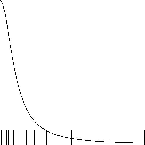
It is also possible to formulate the reverse problem: how to find the sense
$P(x)$ if the density $\{ x_k \}$ has been given. An illustrative
example is the distribution of the tab stops on a guitar's neck. It can be
demonstrated that it is given by:
$$
x_k = L \left( \half \right)^{k/12}
$$
Where $L$ is the length of the strings. The case $x_0$ for $k=0$ corresponds
with the full length of a string. The case $x_{12} = L/2$ for $k=12$ corresponds
with the first octave. And so on. The sequence $x_k$ is monotonically
decreasing for a change. Rewrite the above formula, as follows:
$$
\frac{x_k}{L} = \left( \half \right)^{k/12} \hieruit
\ln \left(\frac{x_k}{L} \right) = \frac{k}{12} \; \ln(\half) \hieruit
- 12 \; ^2\log \left(\frac{x_k}{L} \right) = k
$$
Herewith the problem is squeezed into standard form. And:
$$
\int_L^{x_k} P(t) \, dt = -12 \; \ln \left(\frac{x_k}{L} \right)/\,\ln(2)
\hieruit
\int_x^L P(t) \, dt = 12 \; \ln \left| \frac{x}{L} \right|/\,\ln(2)
$$
The first minus sign stems from the fact that the integration is carried out
in reverse order, from the maximal length of the string downwards to zero (due
to the fact that the sequence is monotonically decreasing).
By differentiating at both sides (and eventually ignoring a minus sign) we
finally find:
$$
P(x) = 12 \; \frac{1/L}{x/L}/\,\ln(2) = \frac{12}{x\;\ln(2)}
$$
So the sense $P(x)$ is independent of the string's length $L$ and it
has a vertical asymptote for $x=0$, where the bridge of the guitar is.
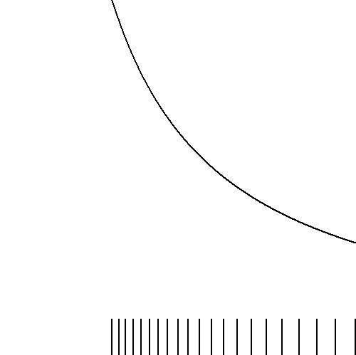
Here is a picture that is relevant for the real thing, with $N=20$ and
$L=1$. Values are not displayed for $k > N$ and $P(x)$ is re-scaled as follows:
$$
P(x_N) = 1 \hieruit P(x) = \frac{D}{x}
\quad \mbox{with} \quad D = \left( \half \right)^{N/12}
$$
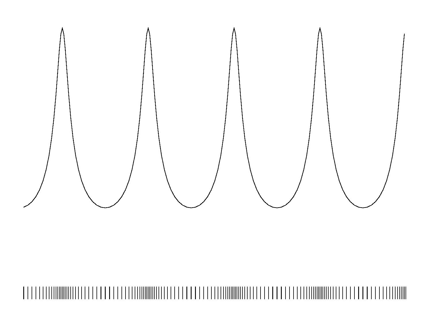
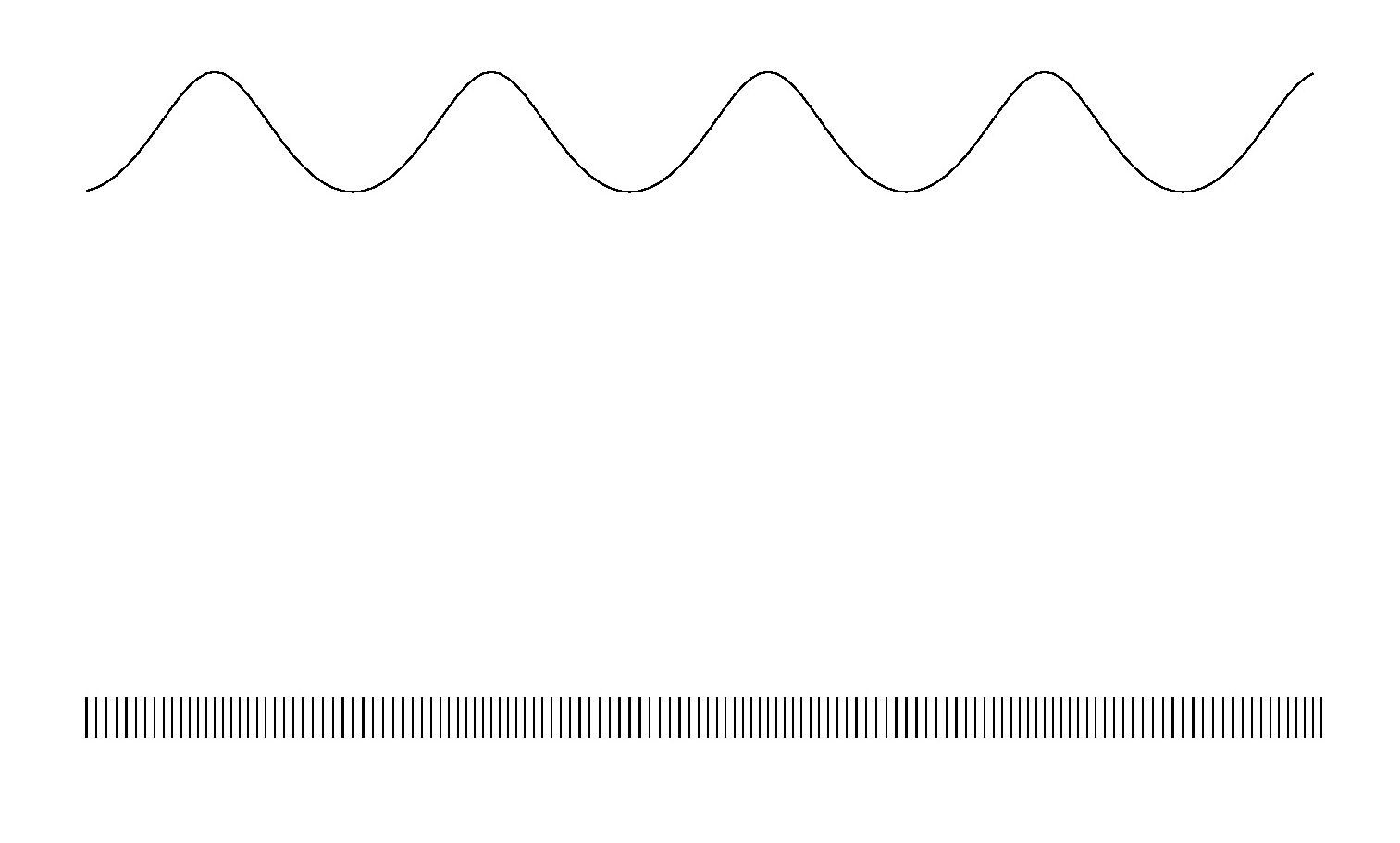
It can be demonstrated experimentally that the sense of a longitudinal
wave - contrary to what might be expected - does not correspond with the
transversal wave from which it has been derived. Strictly spoken, it doesn't
even correspond with a sinusoidal function. Nevertheless, for small amplitudes,
the following approximations shall be made:
$$
x_k = k\,.\,\Delta + A\,.\,\sin\left(\frac{2\pi}{\lambda} k\:\Delta\right)
\hieruit
k\,.\,\Delta = x_k - A\,.\,\sin\left(\frac{2\pi}{\lambda} x_k\right)
$$
The replacement of $(k\Delta)$ by $x_k$ in the above equation is not at all by
accident, though it can only be justified, more or less, if the amplitude $A$
is small enough. By assuming, namely, that $k\Delta \approx x_k$, the sense
function can be found by differentiation:
$$
\int_0^{x_k} P(t) \, dt =
\frac{x_k}{\Delta} - \frac{A}{\Delta}\sin\left(\frac{2\pi}{\lambda} x_k\right)
\hieruit P(x) = \frac{1}{\Delta}\left[1 - A\frac{2\pi}{\lambda}
\cos\left(\frac{2\pi}{\lambda} x\right)\right]
$$
Giving a function $P(x)$ which is indeed maximal where the densities of
the sequence $x_k$ are most dense, as it should be. Such is the case, namely,
at the odd zeroes of the accompanying transversal (sine) wave. Furthermore it
is clear that densities become greater with shorter wavelengths $\lambda$. And,
due to the condition $A < \lambda/(2\pi)$ , the function $P(x)$ is also
positive valued. It should be emphasized again, though, that the assumption
$k\Delta \approx x_k$ is not valid in general, but only as a convenient
approximation for small amplitudes.
Accompanying software for making the pictures is
disclosed as well.