
N = { 1,2,3,4,5, ... }
Theorem. The set of all naturals is a completed infinity.
Proof. A set is infinite (i.e. a completed infinity) if and only if there
exists a bijection between that set and a proper subset of itself.
 |
: one-to-one mapping |
Now consider the even naturals. They are a proper subset of the naturals and a bijection can be defined between the former and the latter. As follows:
  2  4  6  8 10 12 14 16 18 20 22 24 26 28 30 32 34 36 38 ...
  |  |  |  |  |  |  |  |  |  |  |  |  |  |  |  |  |  |  |
  1  2  3  4  5  6  7  8  9 10 11 12 13 14 15 16 17 18 19 ...
According to our first Axiom, such a Completed Infinity, in retrospect, does not exist. Which isn't going prevent anybody from freely employing certain expressions, like for example ( ∀ n ∈ N ), as a well established "figure of speech". So far so good for common mathematics. But how about the mathematics that comes after it? Well, let's take a look at the real world. Especially let's take a look at the mathematics laboratory par excellence, the digital computer. How is "the set of all naturals" represented in there? As numbers running from one up to some maximum integer, usually of order 2^16 or some such. That precise upper bound is not quite relevant. What is relevant is that there is always a limited upper bound to Naturals in practice. Limited sets of naturals are well known in classical mathematics. Any such set is called an initial segment of "the" standard Naturals:
Nn = { 1,2,3,4,5, ... , n }
Each initial segment contains all the naturals, starting from 1 , up to and including a largest natural n . Therefore, with such an initial segment, it does not follow per se that
( a ∈ Nn ) & ( b ∈ Nn ) => (a + b) ∈ Nn
Due to the fact that there is a finite upper bound on the initial segment, the sum (a + b) can be beyond that bound. Which is clearly undesirable. Therefore sort of an idealization is definitely needed, namely such that "beyond a bound" can no longer be the case. A tentative proposal could be to introduce The Naturals as a limit of an initial segment, where the largest natural n approaches infinity. If you don't like this approach, please note that it will lead, in a few steps, to a result which is actually standard mathematics. So you could accept these intermediate steps as sort of heuristic. Whatever, we shall assume, for the moment being, that The Naturals are defined as:
N = limn → ∞ { 1,2,3,4,5, ... , n }
Admittedly, the concept of a limit is somewhat stretched here. What we want to
express is that The Naturals are quite resemblant to an initial segment, apart
from an upper bound. So why not just say that the naturals are an initial
segment without an upper bound. A difference with other approaches is that All
of The Naturals therefore can only be known through its initial segments.
Needless to say that Infinity will never be reached Actually - which is typical
for limits anyway.
A signficant issue in this context is Cardinality. When given a completed
infinity of naturals, a bijection can set up between all naturals and all even
naturals. This is no longer possible when initial segments are the only things
that can be known about the naturals. A bijection can still be set up, but it
does no longer cover "all" naturals in the segment. Instead, bijection reduces
to a process that is known as counting. A count E of the even naturals
in an initial segment where n is even reveals that E = n/2:
  2  4  6  8 10 12 14 16 18 20 22 24 26 28 30 32 ...  n
  |  |  |  |  |  |  |  |  |  |  |  |  |  |  |  |      |
  1  2  3  4  5  6  7  8  9 10 11 12 13 14 15 16 ... n/2 ...
And if n is odd then E = (n-1)/2:
  2  4  6  8 10 12 14 16 18 20 22 24 26 28 30 ... (n-1)
  |  |  |  |  |  |  |  |  |  |  |  |  |  |  |       |
  1  2  3  4  5  6  7  8  9 10 11 12 13 14 15 ... (n-1)/2 ...
Thus, for n is even, we establish the limit
limn → ∞ ( #evens ) / ( # all ) = limn → ∞ ( #{ 1,2,3,4, ... , n/2 } ) / ( #{ 1,2,3,4, ... , n } ) = limn → ∞ n/2 / n = 1/2
And, for n is odd, we establish the limit
limn → ∞ ( #evens ) / ( # all ) = limn → ∞ ( #{ 1,2,3,4, ... , (n-1)/2 } ) / ( #{ 1,2,3,4, ... , n } ) = limn → ∞ (n-1)/2 / n = 1/2
With the quotient of two count functions available, note that it would have been a technicality to define the above tentative limit more rigorously. Indeed, just as with infinitesimals dx and dy , everybody agrees upon the idea that dx and dy may be undefined, but the quotient dy/dx is certainly defined. Whatever. The inevitable conclusion is that the ratio (#evens)/(#all) is equal to 1/2. Thus the "cardinality" of all even naturals divided by the "cardinality" of all naturals is not equal to 1 but equal to 1/2. Mind the scare quotes. Actually the technique as demonstrated is not quite unknown in common mathematics. Look up Natural Density and you will find that it's just like it! So it turns out, in the first place, that no new mathematics is needed. More interesting facts on the Wikipedia webpage "Natural density".
Here we are. Our proposal is thus nothing else than: replace the standard
notion of Cardinality by the other standard notion of Natural Density.
Or rather: leave everything as it is; just consider Natural Densities as more
relevant to the finitistic approach than Cardinalities. This is what I meant,
when I said that an a posteriori judgement can have consequences for
the evaluation of a priori activities.
limn→∞ E(n) / ( n/2 ) = 1
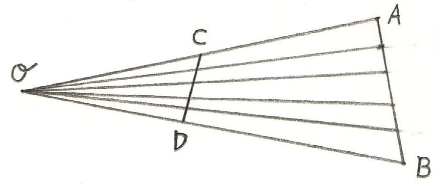
Let π(n) be the number of primes less than n, where n is a natural number.
Then: limn→∞ π(n) / ( n / ln(n) ) = 1
A much less difficult to prove theorem is the following. Let Q(n) be the
number of squares less than or equal to n, where n is is a natural. Then:
limn→∞ Q(n) / ( √n ) = 1 Proof. It's easy to see
that √n - 1 < Q(n) ≤ √n . Now divide by √n to get
1 - 1/√n < Q(n) / ( √n ) ≤ 1 .
For n→∞ the result follows.
Another example. Let B(n) be the number of (positive) fractions (reducible or
not) with denominators and numerators less than or equal to a natural number
n . Then: limn→∞ B(n) / ( n2 ) = 1
though we would rather like to have a formula for irreducible fractions,
of course.
The numerosity (cardinality) of the powers of 7 equals the numerosity of the
naturals. There are as many powers of 7 as there are naturals.
limn→∞ Z(n) / ( log(n) / log(7) ) = 1
[ log = natural logarithm ] Proof. From a picture [ graph of log(x) / log(7) ]
it's easy to see that
Z(n) ≤ log(n) / log(7) < Z(n) + 1 →
log(n) / log(7) - 1 < Z(n) ≤ log(n) / log(7) .
limn→∞ Z(n) / [ A-1(n) ] = 1
Proof. A(n) is monotonically increasing with n , therefore it has an inverse
A-1(n) in the first place.
Thus the gist of the above is not that common mathematics "doesn't know" about
"finitistic cardinalities". It does. And the common theory of cardinalities is
not so much wrong. I'd rather call it redundant. Common mathematics may
be too much of the good. But maybe that redundancy is even inevitable. We shall
see.
PNT look-alikes
One of the most well known theorems in mathematics is the Prime Number Theorem
(PNT).
The Prime Number Theorem has the same form as the trivial statement
that was proved about E(n) = the number of evens, in the previous section:
Proof: there
exists a bijection between the naturals and these powers. As depicted here:
1  2   3    4     5      6      7       8        9        10  ..
|  |   |    |     |      |      |       |        |         |
7 49 343 2401 16807 117649 823543 5764801 40353607 282475249  ..
But let's have another way to look at it:
 1   2 3 4 5 6   7   8 9 10 .. 48  49   50 .. 343 .. 2401 ..
 |               |                  |           |       |
7^0             7^1                7^2         7^3     7^4
Let Z(n) be the number of 7-powers less than or equal to n, where n is a
natural number. Then we have the theorem:
Divide by log(n) / log(7) to get 1 - 1/( log(n) / log(7) ) < Z(n) /
( log(n) / log(7) ) ≤ 1 . For n→∞ the result follows.
Written as an asymptotic identity: Z(n) ~ log(n) / log(7) . Suppose that
A0 is a very large number, then:
Z(A0) = log(A0) / log(7) . Did I suggest anything?
We seek to generalize this result.
   1     2     3     4     5     6    7     8     9   ..
   |     |     |     |     |     |    |     |     |
 A(1)  A(2)  A(3)  A(4)  A(5)  A(6) A(7)  A(8)  A(9)  ..
Let there be defined a function A : N → N on the naturals N.
Examples are the squares [ A(n) = n2 ] and the powers of seven
[ A(n) = 7n ].
And, oh yeah, A(n) is a sequence monotonically increasing with n .
The numerosity / cardinality of the function A(n) equals the numerosity of
the naturals; there are as many values of A as there are naturals.
Proof: there exists a bijection between the naturals and these values,
due to the fact that A(n) is monotonically increasing with n,
thus it has no upper bound, as is the case with the naturals too.
But let's have another way to look at it [ e.g with A(n) = 7n ]:
   1   2 3 4 5 6   7   8 9 10 .. 48  49   50 .. 343 .. 2401 ..
   0   0 0 0 0 0   1   1 1  1     1   2    2      3       4    : Z(n)
 A(0)            A(1)               A(2)        A(3)    A(4)
Let Z(n) be the number of A(m) values (count) less than or equal to n,
where (m,n) are natural numbers. Then we have the following Theorem.
And the inverse A-1(n) is
monotonically increasing as well. Furthermore, we see that Z(n) is m for
A(m) ≤ n < A(m+1) .
Consequently: A(Z(n)) ≤ n < A(Z(n)+1)
→ Z(n) ≤ A-1(n) < Z(n) + 1 →
A-1(n) - 1 < Z(n) ≤ A-1(n)
Divide by A-1(n) to get:
1 - 1 / A-1(n) < Z(n) / A-1(n) ≤ 1 .
For ( n→∞ ) the theorem follows,
because A-1(n) → ∞ .
Written as an asymptotic identity: Z(n) ~ A-1(n) . If A0
is a very large number, then: Z(A0) = A^(-1)(A0)
Examples.
| A(n) = n2 | → | limn→∞ Z(n) / ( √n ) = 1 |
| A(n) = 7n | → | limn→∞ Z(n) / ( log(n) / log(7) ) = 1 |
| A(n) = 2.n | → | limn→∞ Z(n) / ( n/2 ) = 1 |
At the
Wikipedia page about Fibonacci_numbers we find another Asymptotic Equality.
For large n, the Fibonacci numbers are approximately
Fn ~ ( [ 1 + √5 ]/2 )n / √5
Giving a limit similar to the one for the powers of seven:
A(n) = Fn → limn→∞
Z(n) / [ ln(n) / ln( [ 1 + √5 ]/2 ) ] = 1
Calculus XOR Probability
From that wiki page about
Natural Densities a
quote:
We see that this notion can be understood as a kind of probability
of choosing a number, which obviously is the reason why Natural Densities
are studied in probabilistic number theory.
Therefore
another application of the above concepts is with Probability Theory
[ <NL>letter to the editor</NL> ].
Standard mathematics says that it is impossible to have a uniform
probability distribution on the naturals. Meaning that it is impossible to have
a distribution giving equal probabilities to each of (all) the natural numbers.
Not a question, however, about the same for an initial segment of the naturals.
The probability for picking, say, the number 7 out of the initial segment
{ 1,2,3,4,5, ... ,n } is simply: 1/n . The same holds for an arbitrary
number k in that segment. And the sum of all the probabilities is 1/n + 1/n
+ ... + 1/n = n.1/n = 1 , as it should be. But something weird happens if we
take the limit for n → ∞ . Then each of the probabilities for
picking one natural number becomes
limn → ∞ 1/n = 0
while the sum of all probabilities is still 1 , according to
limn → ∞ 1 = 1
How can that happen? A bunch of zeros that sums up to one? Oh well, it's not just a sum of zeros. It's an infinite sum of zeros. But let's take another example, that only seems remotely resemblant. The following very simple integral is expressed as the limit of a Riemann sum.
∫01 dx = limn → ∞ ∑ 1/n = 0 = limn → ∞ ∑1n 1/n = limn → ∞ n.1/n = limn → ∞ 1 = 1
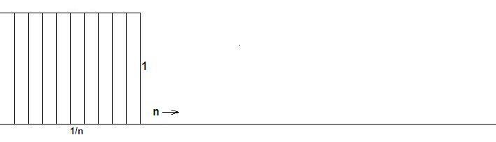
Am I blind or what? The only difference with probabilities is the geometrical
interpretation. Here come the probabilities. It is a histogram with height of
the blocks 1/n and width of the blocks 1 for n blocks. So the total area of
the blocks is (n.1.1/n) = 1 .
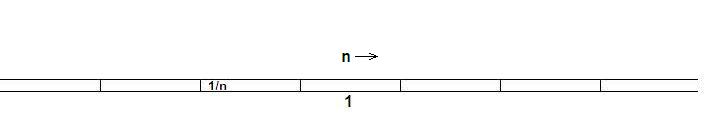
And here comes the Riemann sum of that trivial integral. The blocks are 1/n
wide, 1 high and there are n of them. The total area is (n.1/n.1) = 1 .
Quite obviously, limn → ∞ n.1/n is exactly the same
algebraic expression with the integral as with the probabilities.
But, on the contrary, it is as if they do the following with the probabilities.
limn → ∞ n [ limm → ∞ 1/m ] = limn→∞ n [ 0 ] = 0
First try to define elementary probabilities, check out that they become zero and then sum up. Evidently the sum then becomes zero as well. Instead of:
limn→∞ n [ limn→∞ 1/n ]
I think the twist is clear. But ah, the trouble with understanding this may be
something else, it seems ..
The sum of infinitely many zeros in our tentative probability theory is equal
to one. The Riemann sum in infinitesimal calculus - mind infinitesimal -
is equal to one as well. Could it be that the existence of infinitesimals is
consequently denied in classical mathematics - because especially in calculus
they "aren't needed anymore". As soon as we add a twist to probability theory,
they turn up again. And this time they can no longer be denied or circumvented.
[ No surprise at all for those disciplines where Applied rules the Roast, but
that's another story ] Let's make a brave decision and accept the following
"well known facts" in our AfterMath and perhaps in common mathematics too.
(x = y) ≡ [ ∀ P : P(x) ↔ P(y) ]
I find it somewhat weird that we need sort of an equality ≡ for defining another equality = in terms of a logical equality ↔ . But anyway, let's try some with that definition. Every property in common, they said. We take that quite literally and have, for example:
P(x) ≡ ( x is on the left of the = sign )
With this property in mind, consider the expression:
1 = 1
Then we see that the 1 on the right in 1 = 1 is not on the left, hence the property P(1) as defined does not hold for that one. Consequently: 1 ≠ 1 . We have run into a Paradox. Oh, you should say, but self-referential properties are of course not allowed. Sure, I am the last one to disagree with you. This highly artificial example stresses an important point, though:
( x = y ) ≡ [ ∀ P ∈ I : P(x) ↔ P(y) ]
With an initial segment of the naturals, equality can indeed be established in this way. Let's represent each natural as a bit string, as is quite common with computer representations. Then the aspect I may consist of predicates of the form
Pi(x) = ( bit i of string representing x is up )
And because the initial segment ends, it is clear that the range of indexes i ends as well and hence the set I is finite. So far so good with the naturals, that are representative for the discrete world. Real numbers are representative for the continuous world, though. In the AfterMath, there are limited intervals of the reals, exactly as there are limited intervals of the naturals. Clipping agains a viewport is necessary if the ideal Euclidian Geometry is deemed to be useful with any Computer Graphics application. For the reason that infinitely long straight lines cannot be co-existent with the latter. But, with the real numbers, we have an additional complication. Not only that they have a limited range. In the AfterMath, they also have a limited precision. According to classical mathematics, the real numbers are abundant with irrationals. We can even say that the irrationals form the vast majority of the real numbers. Yet we have equivalents of expressions like x = π or y = √2 in our programming languages, where it is emphasized that the variables x and y, most of the time, have no more than, say, double precision. This is extremely poor, when compared with exact mathematics. Consequently, numbers like π or √2 can by no means be represented exactly with such finite precision, as may be expressed again by an aspect I and its predicates:
Pi(x) = ( bit i of string representing x is up )
We are lucky if all available bits of a mantissa are indeed the binary digits of π or √2. To make life easier, we compute anything in decimal. Let's start with the "exact" value ofd π. Well, not really exact, but far more accurate than with double precision. We invoke MAPLE for that purpose.
> evalf(Pi,30);
                   3.14159265358979323846264338328
With a programming language like Delphi (Pascal), the limitations of double
precision are clearly shown.
program Pie;
begin
  Writeln(Pi:31:29);
end.

D:\jgmdebruijn\Delphi\infinite>Pie
3.14159265358979324000000000000
Compare the two values:
3.14159265358979323846264338328
limx→a f(x) = L
means that f(x) can be made as close to L as desired, by making x sufficiently
close to a, but without actually letting x be a. In this case, we say that
"the limit of f(x), as x approaches a, is L".
The exact definition is as follows. Let f(x) be a function defined on an
interval that contains x = a . Then we say that
limx→a f(x) = L
if x ≠ a and if for every number ε > 0 there is some number
δ > 0 such that
| f(x) - L | < ε
whenever 0 < | x - a | < δ
Note that f(x) is possibly not defined at x = a ; the additional condition
x ≠ a is definitely a refinement.
limn→∞ f(n) = L
means that f(n) can be made as close to L as desired, by making n large
enough. Without actually letting n be ∞ is a trivial addendum in
this case. We say that "the limit of f(n), as n approaches infinity, is L".
The exact definition is as follows. Let f(n) be a function defined for
sufficiently large values of n. Then we say that
limn→∞ f(n) = L
if for every number ε > 0 there is some number N > 0 such that
| f(n) - L | < ε whenever n > N
As an example, consider the following limit:
limn→∞ 1/n
We claim that this limit is equal to zero. Indeed:
| 1/n - 0 | < ε whenever
n > N with N = 1/ε
But without actually letting n to be ∞ . This means that
the limit is not actually reached, quite in concordance with Gauss' dictum.
It has the weird consequence, though, that our zero is not really zero, but
only a limit that approaches zero. With other words, zero is itself but not
itself at the same time. An apparent paradox - and a very old one, if you think
about it. Essentially the famous
"παντα ρει" as uttered by the Greek
philosopher Heracleitos (500 B.C.): "We both step and
do not step in the same rivers. We are and are not."
limn→∞ 1/n
We see, indeed, that the value zero cannot be reached, by far, for the simple
reason that N cannot even be very large on a digital machine (assuming e.g.
standard 16 bits precision for integers):
| 1/n - 0 | < ε whenever
n > N with N = 1/ε
But there is also something very peculiar involved with the reals themselves.
And especially with zero. Remember that other limit definition:
limx→a f(x) = L
if x ≠ a and if for every number ε > 0 there is some number
δ > 0 such that
| f(x) - L | < ε whenever | x - a | < δ
Such numbers ε > 0 and δ > 0 are known in computational
work as errors. However, even the real numbers themselves in a digital
computer are not error free; as is obvious if one seeks to represent irrational
numbers such as π or √2. If x is the floating point number representing
π and δ is the "machine eps" (i.e. an error), then only the following
is true:
x ≠ π and | x - π | < δ
Worse. While carrying out computations with real machine numbers, errors tend
to accumulate. And this is actually reflected within the (ε,δ)
formalism for limits. Let, for example,
|x-a|<δx and |y-a|<δy,
where (a,b) are supposed to be "exact" and (x,y) are machine numbers. Next
calculate
| (x+y) - (a+b) | = | (x-a) + (y-b) | ≤ |x-a| + |y-b| <
δx + δy
So the error in the sum (x+y) is most probably greater than one of the errors
(δx,δy),
namely the sum of these. Similar expressions can easily
be derived for the other elementary operations. And are encountered as well in
common proofs involving limits. We may conclude that the concept of a Limit
actually represents - though idealized - error processing. It is known,
as well, that the overwhelming majority of real numbers in common mathematics
is irrational, that is: they are defined by a limit (e.g. a Cauchy sequence of
some sort). We are ready now, not for the next axiom, but for a rather
Trivial Theorem. Every real number is its own limit
Proof. Consider the identity function: f(x) = x . Then for any real number a :
limx→a f(x) = a . QED.
3.14159265358979324000000000000
The Limit Concept
Suppose f is a real-valued function of x and a is a real number.
The expression
Suppose f is a real-valued function of n , where n is an integer.
The expression
It is utterly trivial
that this dark philosophy will have no consequences at all for those parts of
mathematics where limits play no role. It is almost trivial that this obscure
philosophy has hardly any consequences for the mathematics where only a single
limit, as an end-result, is involved. In this case, it makes little difference
whether that limit is considered as finished or not. Beware, however, because
being an end-result is not easily the case. Most so-called end-results are
meant as building blocks for later use. And as soon as other limits are built
upon such "completed" limits, we surely can have a problem, as we shall
see.
Hence the a posteriori: we cannot know beforehand whether an end-result
will be useful or not as a building block for the next step.
Numerical Substrate
Integer machine numbers are always exact, though not
arbitrary large. Real machine numbers are always approximate (and limited in
size as well). The fact that integer numbers on a computer are not arbitrary
large has consequences for carrying out this limit "in the real world":
Herewith, we have said nothing about
mathematics as a bottom up activity. Who cares that for example the
number 1 actually is a limit? As soon as this limit is finished, then there is
no difference at all between this and a "given" number. As soon as the limit
may be considered as finished, indeed.
Iterated Limits
Little trouble is expected with limits, as long as they are single, that
is: not superposed upon each other. The situation becomes radically different,
however, with repeated or iterated limits.
We start with an example that
could easily come from a standard textbook on calculus.
| F(x,y) = ( x2 - y2 ) / ( x2 + y2 ) | for (x,y) ≠ (0,0) |
| F(x,y) = 0 | for (x,y) = (0,0) |
Let's proceed with some - innocent looking - Iterated Limits.
limx→∞ [ limy→∞
( x2 - y2 ) / ( x2 + y2 ) ] =
limx→∞ [ limy→∞
( x2/y2 - 1 ) / ( x2/y2 + 1 ) ] =
limx→∞ [ -1 ] = -1
limy→∞ [ limx→∞
( x2 - y2) / ( x2 + y2 ) ] =
limy→∞ [ limx→∞
( 1 - y2/x2 ) / ( 1 + y2/x2 ) ] =
limx→∞ [ +1 ] = +1
According to the standard textbook, the iterated limits do not commute.
limx→0 [ limy→0
( x2 - y2 ) / ( x2 + y2 ) ] =
limx→0 [ ( x2 ) / ( x2 ) ] = +1
limy→0 [ limx→0
( x2 - y2 ) / ( x2 + y2 ) ] =
limy→0 [ ( - y2 ) / ( y2 ) ] = -1
So again, according to the textbook, the iterated limits do not commute.
So far so good. We first continue with another standard textbook example.
| Q(x,y) = ( x y ) / ( x2 + y2 ) | for (x,y) ≠ (0,0) |
| F(x,y) = 0 | for (x,y) = (0,0) |
Proceeding again with some - innocent looking - iterated limits:
limx→∞ [ limy→∞
( x y ) / ( x2 + y2 ) ] =
limx→∞ [ limy→∞
( x/y ) / ( x2/y2 + 1 ) ] =
limx→∞ [ 0 ] = 0
limy→∞ [ limx→∞
( x y ) / ( x2 + y2 ) ] =
limy→∞ [ limx→∞
( y/x ) / ( 1 + y2/x2 ) ] =
limx→∞ [ 0 ] = 0
According to the standard textbook, the iterated limits commute.
limx→0 [ limy→0
( x y ) / ( x2 + y2 ) ] =
limx→0 [ limy→0
( y/x ) / ( y2/x2 + 1 ) ] =
limx→0 [ 0 ] = 0
limy→0 [ limx→0
( x y ) / ( x2 + y2 ) ] =
limy→0 [ limx→0
( x/y ) / ( 1 + x2/y2 ) ] =
limx→0 [ 0 ] = 0
According to the standard textbook, the iterated limits commute.
It's good to take a closer look at the above limits.
We will do so by introducing polar coordinates:
x = r cos(φ) y = r sin(φ)
Giving:
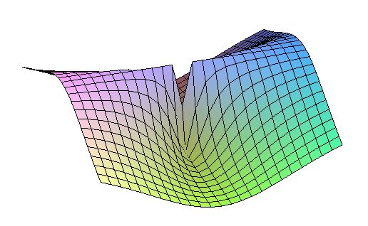
F(x,y) = ( x2 - y2 ) / ( x2 + y2 ) = [ r2 ( cos2(φ) - sin2(φ) ) ] / [ r2 ( cos2(φ) + sin2(φ) ) ] = cos(2φ)
Now we can understand immediately why those limits of F(x,y) for x and y indeed do not commute. At (x,y) = (0,0) this function is singular and it assumes any value between -1 and +1 there. But the latter is the case anywhere else in the (x,y)-plane. A limit for x→∞ and / or y→∞ can assume any value between -1 and +1 as well. Unless there is a clear path to infinity. The function is sort of a circular wave and has a period π . A (MAPLE) picture says more than a thousand words.
> plot3d((x2-y2)/(x2+y2),x=-1..+1,y=-1..+1);
G(x,y) = ( x y ) / ( x2 + y2 ) = [ r2 cos(φ) sin(φ) ] / [ r2 ( cos2(φ) + sin2(φ) ) ] = sin(2φ) / 2
The iterated limits for x and y do indeed commute, but this is more or less a coincidence. In fact, the function G(x,y) is like the function F(x,y) but rotated over an angle of 45o, because sin 2 ( φ - π/4 ) = cos 2φ . Do again the interated limit for G(x,y) while assuming that y=x. The latter is a "clear path" to infinity and to zero. Then we get:
lim(x,y)→(0,0) (x y) / (x2 + y2) = limx→ 0 (x2)(2 x2) = 1/2
lim(x,y)→(∞,∞) (x y) / (x2 + y2) = limx→ ∞ (x2) / (2 x2) = 1/2
Do again the interated limit for G(x,y) while assuming that y = - x , another clear path to infinity and to zero. Then we get:
lim(x,y)→(0,0) (x y) / (x2 + y2) = limx→0 (-x2) / (2 x2 = - 1/2
lim(x,y)→(∞,∞) (x y) / (x2 + y2) = limx→ ∞ (-x2) / (2 x2) = - 1/2
These outcomes are to be expected, because the function G(x,y) is like the
function F(x,y) as described above, apart from a rotation of the coordinate
system. So we can restrict attention to F(x,y), without missing anything.
Now consider again the iterated limits, from an a posteriori viewpoint.
limx→0 [ limy→0 (x2 - y2) / (x2 + y2) ] = limx→0 [ (x2) / (x2) ]
But wait! Here the main axiom comes into effect: Actual Infinity is not given. The limit for y→0 therefore may not be considered as completed. Or the value y = 0 , upon retrospect, is not actually reached: y ≠ 0 . Therefore what's actually left, instead of the number 0 , is a number slightly different from 0 , let's call it epsilon ε :
limx→0 [ limy→0 (x2 - y2) / (x2 + y2) ] = limx→0 [ (x2 - ε2) / (x2 + ε2) ] = limx→0 [ (x2/ε2 - 1) / (x2/ε2 + 1) ] = -1
This is the same outcome as with:
limy→0 [ limx→0 (x2 - y2) / (x2 + y2) ] = limy→0 [ (-y2) / (y2) ] = -1
But wait! Here the main axiom comes into effect: Actual Infinity is not given. The limit for x→0 therefore may not be considered as completed. Or the value x = 0 , upon retrospect, is not actually reached: x ≠ 0 . Therefore what's actually left, instead of the number 0, is a number slightly different from 0, let's call it δ :
limy→0 [ limx→0 (x2 - y2) / (x2 + y2) ] = limy→0 [ (δ2 - y2) / (δ2 + y2) ] = limy→0 [ (1 - y2/δ2) / (1 + y2/δ2) ] = +1
This is the same outcome as with:
limx→0 [ limy→0 (x2 - y2) / (x2 + y2) ] = limx→0 [ (x2) / (x2) ] = +1
We conclude that, from an a posteriori point of view:
limx→0 [ limy→0 F(x,y) ] = limy→0 [ limx→0 F(x,y) ]
But the outcome can be +1 or -1, seemingly at will. Therefore the inevitable
conclusion must be that both limits, actually, do not exist.
We will now prove this in general. The theorem below could have a tremendous
impact upon common mathematical practice, if it were only accepted as true.
Theorem. Iterated limits do always commute. Therefore iterated limits that do not commute do not exist.
Proof. According to the starting hypothesis:
limx→a [ limy→b F(x,y) ] ≠ limy→a [ limx→b F(x,y) ]
According to our a posteriori viewpoint:
limx→a [ limy→ b F(x,y) ] = limx→a F(x,b+ε) = F(a+δ,b+ε)
On the other hand:
limy→b [ limx→a F(x,y) ] = limy→b F(a+δ,y) = F(a+δ,b+ε)
Consequently:
limx→ a [ limy→b F(x,y) ] = limy→ b [ limx→a F(x,y) ]
Because the limits are not really reached. So iff they exist, then thus
they must be identical. This already completes the proof, by contradiction.
Note. The reverse is not true. Limits that do commute (by "coincidence")
do not necessarily exist. An example is the function G(x,y) above, which is
essentially identical to its counterpart F(x,y), apart from a rotation and a
scaling.
The sinc function
Quite useful in physics applications (e.g. optics) is the so-called sinc
function - an old friend of mine, which is commonly
defined as follows:
| sinc(x) | = sin(x) / x | for x ≠ 0 |
| = 1 | for x = 0 |
The function is continuous (and differentiable) everywhere. Especially it is continuous at x = 0 . Proof of the latter rests on a well known limit:
limx→0 sin(x) / x = 1 = sinc(0)
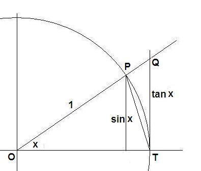
A part of the unit circle is shown.
From the picture it is clear that: triangle area (OTP) < circle sector (OTP)
< triangle area (OTQ). Algebraically this is translated into
sin(x)/2 < x/2 < tan(x)/2 ↔ 1 < x/sin(x) < 1/cos(x) ↔ cos(x) < sin(x)/x < 1
For x→0 not only the right hand side is 1 but the left hand side becomes 1 as well: limx→0 cos(x) = 1 . The sinc function thus becomes trapped between two values equal to 1 . Therefore it can itself be nothing else than 1 . Mind, however, that the value x = 0 is never reached. This brings us to the following alternative definition. Oh yes, among numerous other possibilities, but this one will do.
| sinc(x) | = sin(x) / x | for x ≠ 0 |
| = 2 | for x = 0 |
Would such a definition be possible? In a mathematics with completed infinities the answer is certainly yes. Because we already have all those real numbers in the first place, each of them as a completed entity i.e. finished limits. But here exactly is the vemin! When establishing the continuity of our friend the sinc function, the former limits - necessary to obtain the real numbers - are intermixed with the latter limit, the one for establishing continuity. Thus what we actually have is an iterated limit. Which, as we have seen in the previous subsection, may be quite another matter. Taking one step back - Infinitum Actu Non Datur - this is the content of the Trivial Theorem that any real number is the limit of itself:
| sinc(x) | = sin(x) / x | for x ≠ 0 |
| = 2 | for x = 0 |
| x = 0 ↔ | limx→0 x = 0 | ↔ | x - 0 | < δ | where x ≠ 0 |
| y = 1 ↔ | limy→1 y = 1 | ↔ | y - 1 | < ε | where y ≠ 1 |
To be compared with:
limx→0 sin(x) / x = 1
Taking one step back, this is all there is:
| x - 0 | < δ → | sinc(x) - 1 | < ε
In view of the Trivial Theorem equivalent with:
x = 0 → sinc(x) = 1
The former is continuity for sinc(x), the latter is equality for sinc(x).
What's really happening here is that the limit of a real number definition and
the limit defining continuity are messing up. In fact, there is just one
single limit. In fact, the real numbers are always part of continuity,
real numers are continuous numbers. As an immediate consequence, we must admit
that a definition like sinc(0) = 2, though "possible" in traditional theory,
is utterly nonsensical.
Theorem. It is impossible to have a definition for the value of the
sinc function at x = 0 other than sinc(0) = 1.
Therefore we can simply
define it as follows. All the rest is a mere consequence of this definition.
sinc(x) = sin(x) / x → sinc(0) = 1
Also with constructivist mathematics, there doesn't exist such a choice between sinc(0) = 2 or sinc(0) = 1. The mere fact that sinc(x) is a real valued function guarantees that, for x = 0 , sinc(x) = 1 must hold. According to Brouwer's Continuity Theorem, other values are simply not possible. And again, this is entirely in agreement with physical reality as well.