Efficient 2-D & 3-D Point Probes

Very much improved (2021) program sources and results found at the bottom lines of:

• Voronoi & Delaunay Software
Repeated here for convenience:
• Unit1.pas Theory at Mathematics Stack Exchange:
Is there any equation for triangle? or the backup of it
Converting triangles to isosceles, equilateral or right??? or the backup of it

Here is an animation of finding the triangle where a target point (red ball) is in.
A proper function value at the target shall be obtained by linear interpolation.

Accompanying theory is not much different from the one below, though.

Given a point ('probe') with coordinates $(a,b,c)$. Given a (discretized) field where function values $f(x_k,y_k,z_k)$ are known (: at nodal point positions $k$ ).
What is the value of $f(a,b,c)$, at the probe's position ?

Inside / Outside

Let the shape functions of a (say linear) element be called $N_k$ .
Then an Inside/Outside function is associated with the element, which is defined as:
$\operatorname{IO}(\xi,\eta,\zeta) = $ minimum of $N_k(\xi,\eta,\zeta)$ , where $(\xi,\eta,\zeta)$ are local coordinates.
For $\operatorname{IO}(\xi,\eta,\zeta) \gt 0$ a point $(\xi,\eta,\zeta)$ is inside the element.
For $\operatorname{IO}(\xi,\eta,\zeta) \lt 0$ a point $(\xi,\eta,\zeta)$ is outside the element.
For $\operatorname{IO}(\xi,\eta,\zeta) = 0$ a point $(\xi,\eta,\zeta)$ is at the element's boundary.

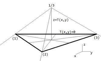
Let's take a look at the IO function of a triangle. We have learned that it's shape functions are given by: $$ \xi = \begin{vmatrix} x-x_1 & x_3-x_1 \\ y-y_1 & y_3-y_1 \end{vmatrix} / \Delta \quad ; \quad \eta = \begin{vmatrix} x_2-x_1 & x-x_1 \\ y_2-y_1 & y-y_1 \end{vmatrix} / \Delta \\ \Delta = \begin{vmatrix} x_2-x_1 & x_3-x_1 \\ y_2-y_1 & y_3-y_1 \end{vmatrix} $$ $$ N_1(\xi,\eta) = \xi \quad ; \quad N_2(\xi,\eta) = \eta \quad ; \quad N_3(\xi,\eta) = 1-\xi-\eta $$ $$ \operatorname{IO}(\xi,\eta) = \operatorname{min}(\xi,\eta,1-\xi-\eta) $$ The maximum of the IO function is reached for $\;\xi=\eta=1-\xi-\eta\;\rightarrow\; = 1/3$ , hence at the midpoint (barycenter) of the triangle. If we draw straight lines from the the midpoint towards the vertices, and further, then the whole plane is subdvided into three regions, one where IO $ = \xi$ , one where IO = $\eta$ and one where IO $= 1-\xi-\eta$ . The IO function is zero at the triangle edges, positive inside and negative outside. It's shaped like a mountain with top $1/3$ at the midpoint and three sharply edged slopes downhill. The contour lines of this function are triangles, where the isoline at xontour level $0$ is the original triangle itself. Hope you get the picture ;-)

Let's take a look at the IO function of a tetrahedron now. It's shape functions are given by: $$ \xi = \begin{vmatrix} x-x_1 & x_3-x_1 & x_4-x_1 \\ y-y_1 & y_3-y_1 & y_4-y_1 \\ z-z_1 & z_3-z_1 & z_4-z_1 \end{vmatrix} / \Delta \quad ; \quad \eta = \begin{vmatrix} x_2-x_1 & x-x_1 & x_4-x_1 \\ y_2-y_1 & y-y_1 & y_4-y_1 \\ z_2-z_1 & z-z_1 & z_4-z_1 \end{vmatrix} / \Delta $$ $$ \zeta = \begin{vmatrix} x_2-x_1 & x_3-x_1 & x-x_1 \\ y_2-y_1 & y_3-y_1 & y-y_1 \\ z_2-z_1 & z_3-z_1 & z-z_1 \end{vmatrix} / \Delta \quad ; \quad \Delta = \begin{vmatrix} x_2-x_1 & x_3-x_1 & x_4-x_1 \\ y_2-y_1 & y_3-y_1 & y_4-y_1 \\ z_2-z_1 & z_3-z_1 & z_4-z_1 \end{vmatrix} $$ $$ N_1 = \xi \quad ; \quad N_2 = \eta \quad ; \quad N_3 = \zeta \quad ; \quad N_4 = 1-\xi-\eta-\zeta $$ $$ \operatorname{IO}(\xi,\eta,\zeta) = \operatorname{min}(\xi,\eta,\zeta,1-\xi-\eta-\zeta) $$ The maximum of the IO function is reached for $\;\xi=\eta=\zeta=1-\xi-\eta-\zeta\;\rightarrow\; = 1/4$ , hence at the midpoint (barycenter) of the tetrahedron. If we draw straight lines from the the midpoint towards the vertices, and further, then the whole space is subdvided into four regions, one where IO $ = \xi$ , one where IO = $\eta$ , one with IO $= \zeta$ , and one where IO $= 1-\xi-\eta-\zeta$ . The isosurfaces of this function are tetrahedra, where the isosurface at level $0$ is the original tetrahedron itself. Hope you get the 4-D picture ;-)

Back to the 2-D case. Instead of the brute force approach, that is simply test if IO$(a,b) \ge 0$ for each triangle, a much more sophisticated search procedure now comes into mind. Determine the slope where the probe point is 'sliding' on. If for example IO $= \xi$ , which is the shape function belonging to vertex (1), then the probe must be searched in the direction (2)-(3). In general, if the IO function equals the shape function belonging to vertex (k), then searching must proceed in the direction of the other two vertices. Stated more explicitly: the next triangle to be investigated is the one that has these two other vertices in common with the present triangle. This in turn means that we should be able to lookup quickly vertex points in the connectivity array, preferrably without having to transverse the whole array.

In fact we have an inverse problem. The connectivity array determines the vertex points belonging to a given triangle. What we need here instead is to know which triangles are the neighbors of a given triangle. A general solution to this problem would consist in constructing the inverse topology, also called 'dual' connectivity. This is almost equivalent with saying that the Voronoi regions of a (Delaunay) triangulation are to be constructed. Programming details for the newest version are in Voronoi & Dekaunay, especially the Shamos module with the 'Duaal' routine in it.

Fortran details deprecated

An additional array DONE keeps track of the elements which have been handled. It may happen that the search path ends before a suitable element has been found. This will repeatably be the case with non-convex area's / volumes. In that case the search procedure will be restarted with an element which has not been DONE already. The search procedure is restarted every time an element is encountered which has been DONE : it has no sense to continue a deterministic process, the outcome of which is known. This may happen until all elements are exhausted. At last, the probe point may be outside the mesh. So our efficient probe algorithm may turn out to be equivalent to the brute force method, in the end. But it will never be less efficient than this. Most of the time, the overall gain in efficiency will be considerable. In the 3-D case, say with 1000 elements in a convex region, it may be possible to localize the probe point within approximately 10 steps.
Even real-time performance should be within the realm of posibilities: using the current tetrahedron as the one to begin with, the next tetrahedron to be probed can be found almost immediately by the above algorithm.

Two Fortran programs were developed, meant as an implementation of the above. The 2-D and 3-D programs work with coordinates and connectivity data. These are the files 'coor2d.dat' or 'coor3d.dat' and 'topol2d.dat' or 'topol3d.dat' respectively. Sample data can be generated by a random coordinates generator and a 2-D or 3-D Delaunay 'triangulator', as follows:

 fc Random.FOR
 a.out
 # Outputs: 't' , 'coor2d.dat' , 'coor3d.dat'
 voronoi -t < t > topol2d.dat
 tetras < coor2d.dat > topol3d.dat

 fc suna57a.FOR -o probe2d
 probe2d 0.5 0.5

 fc suna57b.FOR -o probe3d
 probe3d 0.5 0.4 0.6

Visualization of the search process is feasible for the 2-D case. A little post-processing program was developed for this purpose. At first, standard output has to be re-directed to a file named 'found2d.dat'. Then the program must be loaded, together with a PostScript initialization routine, a drawing routine and a routine for minimizing numerical output. At last the whole thing is executed and the result may be enjoyed at the screen and/or spooled to a PostScript printer. (Search path is painted gray, target triangle is painted black. And I'm too lazy to debug the random gray lines ... ;-)

 probe2d 0.5 0.5 > found2d.dat
 fc Letsee.FOR plots.FOR plot.FOR log10.FOR -o Letsee
 Letsee
 gs meshpath.ps
 lpr -Pps meshpath.ps

  Random.FOR:   parameter (LIMIT=20)
 suna57b.FOR:   parameter (LIMIT=25,MANY=75)
 suna57a.FOR:   parameter (LIMIT=100,MANY=187)
  Letsee.FOR:   parameter (NODES=1500,LINES=4500)