Voronoi & Delaunay

We like to continue the story in the previous section with an outstanding example of Specification: the Voronoi diagram.
The (first order logic) predicate that defines a Voronoi region is found in Voronoi Diagrams and Delaunay Triangulations, O'Rourke, Chapter 5 slide 12/52:
Definition:
Given points $P = \{p_1,\cdots,p_n\}$ the Voronoi region of point $p_i$, $V(p_i)$ is the set of points at least as close to $p_i$ as to any other point in $P$: $$ V(p_i) = \left\{x \left|\;|p_i-x| \le |p_j-x| \right. \;\forall \, 1 \le j \le n \right\} $$ Written as a Boolean function in (Delphi) Pascal we have the following code snippet.

function Voronoi(site : integer; x,y : double) : boolean;
{
  Voronoi region that
  belongs to a (site)
}
var
  N,k : integer;
  x1,x2,y1,y2,xm,ym,f : double;
  OK : boolean;
begin
  N := Length(rij);
  OK := true;
  x1 := rij[site].x; y1 := rij[site].y;
  for k := 0 to N-1 do
  begin
    if k = site then Continue;
    x2 := rij[k].x; y2 := rij[k].y;
  { For all Perpendicular Bisectors }
    xm := (x1+x2)/2; ym := (y1+y2)/2;
    f := (x-xm)*(x2-x1)+(y-ym)*(y2-y1);
    OK := OK and (f < 0);
  end;
  Voronoi := OK;
end;

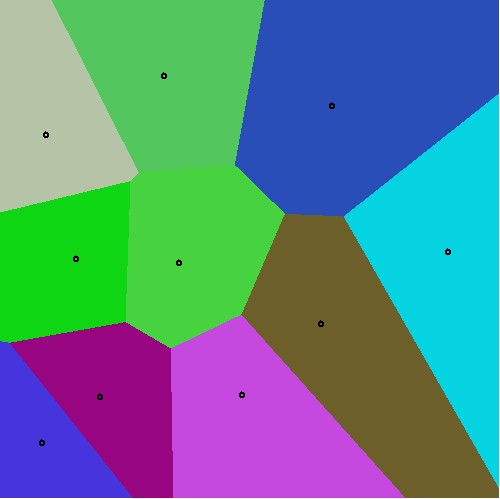
With the previous section in mind, it has become a matter of routine to visualize the accompanying regions as a partition of subsets of the computer screen at hand:

The above is part of a whole bunch of Voronoi & Delaunay activities which took place in November 2021.
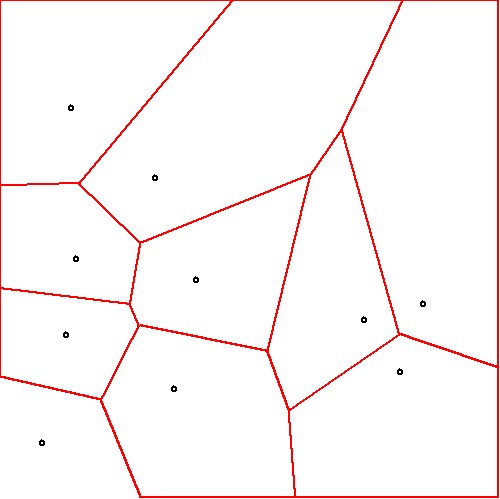
A major lesson is that making a Delaunay Triangulation out of Voronoi Regions is not as simple in practice as it seems to be in theory. First step is to delineate the regions with Isolines/Contours. The next step is recognition of the straight lines, which in theory can be done with Fan Data Compression. Then we can draw perpendiculars from the sites onto those straight lines and we should obtain sort of a Delaunay triangulation. The pictures below show that practice is not quite close to theory. Screen pixels are not small enough for the purpose of obtaining a decent approximation.

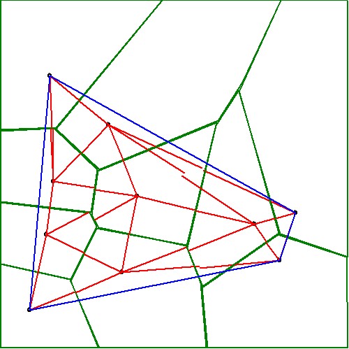
The reverse procedure - obtaining Voronoi Regions out of a Delaunay Triangulation - is easier to do and much more accurate:

A major lesson to be drawn from the latter, however, is that the boundary - a convex hull in our case - is rather tricky. Triangles with sides at the hull can not be handled on the same footing as triangles inside the bulk of the mesh. Details are found in the programming.
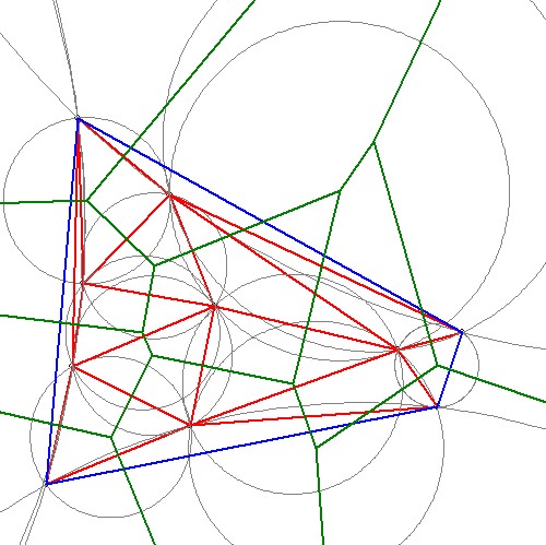
Obtaining an efficient computation of the Delaunay Triangulation is a challenge as such. I have developed a supposedly new method for doing this, which is claimed to have an efficiency $O(n^2)$, while the brute force method adopted at an earlier stage is only $O(n^4)$. The new method works by starting at the hull and proceeding towards the inside of the mesh to be formed. It seems that the most appropriate data structure for such a procedure has to be based upon (oriented) edges instead of triangles. The usual connectivity of a triangular mesh is recovered only at the last step. Here is an animation of the method.

Becoming off-topic more and more; therefore the story is continued at : What is the proper way to do DTFE .