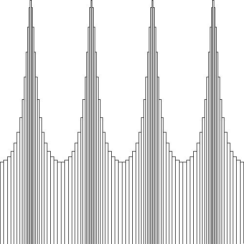
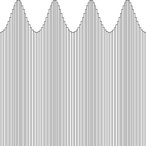
A piecewise constant distribution can also be defined as follows, which is more convenient with regard to other developments: $$ \Pi_k(x) = \left\{ \begin{array}{ll} 0 & \mbox{for} \quad x < x_{k-1} \\ 1/(x_{k+1}-x_k) & \mbox{for} \quad x_{k} \le x \le x_{k+1}\\ 0 & \mbox{for} \quad x > x_{k+1} \end{array} \right. $$ And: $$ P(x) = \sum_{k=1}^N \Pi_k(x) $$ As a next step, approximate the function values $P_k$ by employing a piecewise linear interpolation. First define the following function, which has the shape of a triangle with base $(x_{k+1}-x_{k-1})$: $$ \Delta_k(x) = \left\{ \begin{array}{ll} 0 & \mbox{for} \quad x \le x_{k-1} \\ 2 (x-x_{k-1}) / \left[ (x_k-x_{k-1})(x_{k+1} - x_{k-1})\right] & \mbox{for} \quad x_{k-1} \le x \le x_k \\ 2 (x_{k+1}-x) / \left[ (x_{k+1}-x_k)(x_{k+1} - x_{k-1})\right] & \mbox{for} \quad x_k \le x \le x_{k+1} \\ 0 & \mbox{for} \quad x \ge x_{k+1} \\ \end{array} \right. $$ In such a way namely that, for each of the triangles $\Delta_k$, the area underneath is equal to one. The base of each triangle being $(x_{k+1}-x_{k-1})$ and its height $2/(x_{k+1}-x_{k-1})$. The sense as a whole is given by: $$ P(x) = \sum_{k=1}^N \Delta_k(x) $$ It is noticed that $\sum_k \Delta_k(x)$ will remain zero at the end-points, that is for $k = 1$ and $k = N$. Therefore $P(x)$ will be very steep in that neighbourhood. But nevertheless, this sense function approximation is continuous everywhere:
At last, we might try an approach as in Uniform Combs
of Hat Functions, especially the one with Gaussians:
$$
P(x) = \sum_{L=-\infty}^{+\infty} p(x-L.\Delta)\,\Delta
\MET p(x) = \norm e^{-\half\left(x/\sigma\right)^2}
$$
It is shown in the Gaussians chapter that, in order to achieve sufficient continuity,
the spread $\sigma$ of the bell shapes must be according to:
$$
\sigma > \frac{\Delta}{2\pi}\sqrt{2\:\ln(2/\epsilon)}
$$
where $\Delta$ is the (uniform) discretization and $\epsilon$ is an error,
say $\epsilon=1/256$.
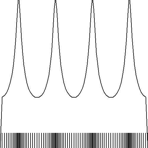
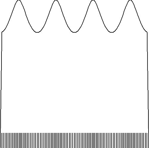
With non-uniform grids, it is suggested - quite analogous with the histogram approximation -
that the above uniform Gaussian sense shall be replaced by the following non-uniform one:
$$
P(x) = \sum_{k=0}^N p_k(x)
\MET p_k(x) = \frac{1}{\sigma_k\sqrt{2\pi}}\, e^{-\half\left[(x-\mu_k)/\sigma_k\right]^2} \\
\Delta_k = x_{k+1}-x_k \quad ; \quad \mu_k = \half(x_{k+1}+x_k)
\quad ; \quad \sigma_k = \frac{\Delta_k}{2\pi}\sqrt{2\:\ln(2/\epsilon)}\times 2
$$
It is noticed that each of the Gaussians $p_k(x)$ has an area $=1$ underneath, just as with
the histograms. That's the reason why a factor $\Delta_{(k)}$ has disappeared in the non-uniform version.
But why the factor $\times 2$ in the end? Well, that's an experimental issue which is
not at all clear to me: it just seems that the original $\sigma_k$ estimates are not big enough for
some reason.
But anyway, here is the graphical result, for (small) $N=25$ and the longitudinal wave example:
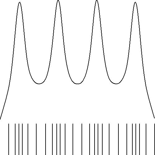
Accompanying software for making the pictures is disclosed as well.