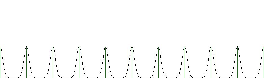
Such combs are defined as:
$$
P(x) = \sum_{L=-\infty}^{+\infty} p(x-L.\Delta)\,\Delta
$$
Where $\Delta$ is the discretization interval length and where being
normed means that:
$$
\int_{-\infty}^{+\infty} p(x)\,dx = 1
$$
In addition, all hat functions are assumed to be symmetrical around
$x = 0$:
$$
p(-x) = p(x)
$$
Given a sufficient refinement of the discretization $\Delta$ - to be defined
later - the comb $P(x)$ can be interpreted as a Riemann sum, approximating the
following integral, with $\Delta \rightarrow d\xi$. This explains the factor
$\Delta$ in the above definition.
$$
\lim_{\Delta \rightarrow 0} P(x) =
\int_{-\infty}^{+\infty} p(x-\xi)\,d\xi = 1
$$
The function $P(x)$ can be interpreted as an attempt to "smooth" the uniform
density $x_L = L.\Delta$. Or "make fuzzy" the discretization $f(x_L) = 1$ of
a constant - and continuous - function $f(x) = 1$. This could be called the
Special Theory of Continuity.
It is easily shown that the above function $P(x)$ is periodic. Its period
is equal to $\Delta$: $P(x + \Delta) = P(x)$ for arbitrary $x$. Meaning that
$P(x)$ can be developed into a Fourier series. The Fourier series of any
periodic function is given by:
$$
P(x) = \half a_0 + \sum_{k = 1}^{\infty} a_k \, cos(k \omega x)
$$
But, in addition, the function is even, meaning that $P(x)=P(-x)$, which
results in real-valued Fourier coefficients $a_k$ :
$$
a_k = \frac{1}{\Delta/2} \int_{-\Delta/2}^{+\Delta/2}
P(x) \cos(k \: 2 \pi / \Delta \, x) \, dx
$$
In the sequel, kind of an angular frequency $\omega$ will stand for the
quantity $ = 2\pi/\Delta$. Then let the calculations continue:
$$
= \frac{1}{\Delta/2} \int_{-\Delta/2}^{+\Delta/2}
\sum_{L = -\infty}^{+\infty} p(x - L \Delta)\,\Delta \cos(k\omega x) \, dx
$$ $$
= 2 \times \sum_{L = -\infty}^{+\infty} \int_{-\Delta/2}^{+\Delta/2}
p(x - L \Delta) \cos(k\omega x) \, dx
$$
Substitute $y = x - L \Delta$ and integrate to $y$:
$$
a_k/2 = \sum_{L = -\infty}^{+\infty}
\int_{- \Delta/2 - L \Delta}^{+ \Delta/2 - L \Delta}
p(y) \cos(k \omega [y + L \Delta]) \, dy
$$
Where:
$$
\cos(k\omega [y + L \Delta]) = \cos(k\omega y + k.L.2\pi) = \cos(k\omega y)
$$
Next replace $y$ by $-y$ and switch integration bounds:
$$
a_k/2 = \sum_{L = -\infty}^{+\infty}
\int_{L \Delta - \Delta/2}^{L \Delta + \Delta/2}
p(y) \cos(k \omega y) \, dy
$$
The above integrals are precisely the adjacent pieces of another integral which
has bounds reaching to infinity. That is, they sum up to an infinite integral:
$$
a_k/2 = \int_{- \infty}^{+ \infty} p(y) \cos(k \omega y) \, dy
$$
Now the (continuous) Fourier integral of $p(x)$ is defined by:
$$
A(y) = \int_{- \infty}^{+ \infty} p(x) \cos(x y) \, dx
$$
Wherefrom it is concluded that the (discrete) coefficients of the Fourier
series are a sampling of the (continuous) Fourier integral:
$$
a_k/2 = A(k \omega)
$$
And especially:
$$
a_0/2 = A(0) = \int_{- \infty}^{+ \infty} p(x) \, dx \hieruit \half a_0 = 1
$$
Therefore the general expression for the Fourier series of a uniform comb of
hat functions is:
$$
P(x) = 1 + 2 \times \sum_{k = 1}^{\infty} A(k \omega) \, cos(k \omega x)
$$
Where it is reminded that $\omega = 2\pi / \Delta$. And:
$$
A(y) = \int_{- \infty}^{+ \infty} p(x) \cos(x y) \, dx
$$
It is seen herefrom that $P(x)$, indeed, is an approximation of the constant
function $f(x) = 1$, provided that the rest of the Fourier series is just a
minor correction on this value. At hand of a few sample hat functions $p(x)$,
we will investigate if such is the rule, rather than an exception.