The OP's equation is:
$$
a(x,y)\frac{\partial^2 u}{\partial x^2}+b(x,y) \frac{\partial^2 u}{\partial y^2}
+c(x,y)\frac{\partial^2 u}{\partial x \partial y}\\+d(x,y)\frac{\partial u}{\partial x}
+e(x,y)\frac{\partial u}{\partial y}+f(x,y)u=g(x,y)
$$
But, for some good reasons, we shall consider instead:
$$
\begin{bmatrix} \partial / \partial x & \partial / \partial y \end{bmatrix}
\begin{bmatrix} A(x,y) & C(x,y) \\ C(x,y) & B(x,y) \end{bmatrix}
\begin{bmatrix} \partial u / \partial x \\ \partial u/ \partial y \end{bmatrix}\\
+D(x,y)\frac{\partial u}{\partial x}+E(x,y)\frac{\partial u}{\partial y}+F(x,y)u=G(x,y)
$$
Seeking for similarities:
$$
\frac{\partial}{\partial x}\left[A(x,y)\frac{\partial u}{\partial x}+C(x,y)\frac{\partial u}{\partial y}\right]+
\frac{\partial}{\partial y}\left[C(x,y)\frac{\partial u}{\partial x}+B(x,y)\frac{\partial u}{\partial y}\right]\\
+D(x,y)\frac{\partial u}{\partial x}+E(x,y)\frac{\partial u}{\partial y}+F(x,y)u=G(x,y) \quad \Longleftrightarrow \\
A\frac{\partial^2 u}{\partial x^2}+B\frac{\partial^2 u}{\partial y^2}+2C\frac{\partial^2 u}{\partial x \partial y}\\
+\left[\frac{\partial A}{\partial x}+\frac{\partial C}{\partial y}+D\right]\frac{\partial u}{\partial x}
+\left[\frac{\partial C}{\partial x}+\frac{\partial B}{\partial y}+E\right]\frac{\partial u}{\partial y}+Fu=G
$$
we conclude that the OP's equation can be rewritten as:
$$
\begin{bmatrix} \partial / \partial x & \partial / \partial y \end{bmatrix}
\begin{bmatrix} a & c/2 \\ c/2 & b \end{bmatrix}
\begin{bmatrix} \partial u / \partial x \\ \partial u/ \partial y \end{bmatrix}
+D\frac{\partial u}{\partial x}+E\frac{\partial u}{\partial y}+fu=g
$$
provided that:
$$
D = d(x,y)-\left[\frac{\partial a}{\partial x}+\frac{\partial c}{\partial y}\right] \quad ; \quad
E = e(x,y)-\left[\frac{\partial c}{\partial x}+\frac{\partial b}{\partial y}\right]
$$
With these modifications, the equation is suitable for
numerical treatment.
We only have to "downsize" the numerical method in the
accompanying document
from 3-D to 2-D.
The terms $\,+fu=g\,$ are easy, so we shall do them first.
It is argued in this
answer @ MSE
that integration (points) at the vertices of a finite element are often the best.
Accompanying pictures are inserted here too for convenience:
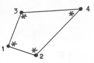
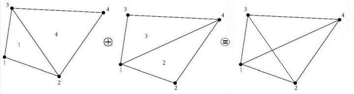
An interesting consequence is splitting of the quadrilateral in four linear triangles:
This makes the discretization of the terms $\,+fu=g\,$ extremely simple:
$$
+ \frac{1}{4} \begin{bmatrix} f_1\cdot\Delta_1 & 0 & 0 & 0 \\
0 & f_2\cdot\Delta_2 & 0 & 0 \\
0 & 0 & f_3\cdot\Delta_3 & 0 \\
0 & 0 & 0 & f_4\cdot\Delta_4 \end{bmatrix}
\begin{bmatrix} u_1 \\ u_2 \\ u_3 \\ u_4 \end{bmatrix} =
\frac{1}{4} \begin{bmatrix} g_1\cdot\Delta_1 \\ g_2\cdot\Delta_2 \\ g_3\cdot\Delta_3 \\ g_4\cdot\Delta_4 \end{bmatrix}
$$
Here $\Delta_k$ is twice the area of the triangle numbered as $(k)$.
The diffusion term has the form:
$$
\frac{\partial Q_x}{\partial x} + \frac{\partial Q_y}{\partial y}
$$
with
$$
\begin{bmatrix} Q_x \\ Q_y \end{bmatrix} =
\begin{bmatrix} a & c/2 \\ c/2 & b \end{bmatrix}
\begin{bmatrix} \partial u / \partial x \\ \partial u/ \partial y \end{bmatrix}
$$
If $\,u\,$ is interpreted as a temperature then this may be considered as a heat flow $\,\vec{Q}\,$
in a medium with anisotropic conductivity.
In this way, the diffusion term can be treated with the standard Galerkin method, exactly as in the abovementioned
reference, or according to an answer
at MSE
with very much the same content.
With help of the differentiation matrix, for each (of the four !) triangles in our basic quadrilateral, the $3 \times 3$ Finite Element matrix for diffusion alone
is like this, with $\Delta/2 = $ area of a triangle : $\Delta/4 \times$
$$ -
\begin{bmatrix} (y_2 - y_3) & -(x_2 - x_3) \\
(y_3 - y_1) & -(x_3 - x_1) \\
(y_1 - y_2) & -(x_1 - x_2) \end{bmatrix} / \Delta
\begin{bmatrix} a & c/2 \\ c/2 & b \end{bmatrix}
\begin{bmatrix} +(y_2 - y_3) & +(y_3 - y_1) & +(y_1 - y_2) \\
-(x_2 - x_3) & -(x_3 - x_1) & -(x_1 - x_2) \end{bmatrix} /\Delta
$$
And take notice of the minus sign!
The Finite Element
assembly scheme
is thus employed at an elementary level, using the topology:
1 2 3 2 4 1 3 1 4 4 3 2
Our Ansatz for the advection element matrix resembles the one for diffusion, but without the OP's $(a,b,c)$ tensor:
$$
M = - \frac{\Delta}{4} \times
\begin{bmatrix} +(y_2 - y_3) & -(x_2 - x_3) \\
+(y_3 - y_1) & -(x_3 - x_1) \\
+(y_1 - y_2) & -(x_1 - x_2) \end{bmatrix} / \Delta
\begin{bmatrix} +(y_2 - y_3) & +(y_3 - y_1) & +(y_1 - y_2) \\
-(x_2 - x_3) & -(x_3 - x_1) & -(x_1 - x_2) \end{bmatrix} /\Delta
$$
Now determine the values of $D(x,y)$ and $E(x,y)$ at the midpoints $(x,y)$ of each of the triangle edges
$(i,j) = (1,2) \to (2,3) \to (3,1)$ and form the inner products:
$$
P_{ij} = D(x,y)(x_j-x_i)+E(x,y)(y_j-y_i)
$$
Then multiply these contributions with the Ansatz, while using an
upwind scheme ,
for $i \ne j$ :
$$
M_{ij} := M_{ij}\times\max(0,-P_{ij}) \quad ; \quad M_{ji} := M_{ji}\times\max(0,-P_{ji})
$$
The main diagonal terms must be made equal to minus the sum of the off-diagonal terms in order to finish the advection matrix.
Does the above sound a bit improbable? The secret behind it is in the section Voronoi Regions
of the 2-D reference.
There we find the following formula for the resistor ($R_3$) equivalent of diffusion:
$$
R_3 = \frac{ \mbox{"length" of } R_3 }{ \mbox{conductivity} \, \times \, \mbox{"diameter" of } R_3 }
$$
Turning it upside down and leaving out the conductivity - as has been done - we have for the Ansatz:
$$
\mbox{matrix entry} = \frac{\mbox{"diameter" of edge}}{\mbox{"length" of edge}}
$$
This is multiplied with the inner product of a "velocity" and an edge,
thus resulting in a "flux", being the projection of a "velocity" times the diameter ("area") of the edge.
At last all elementary parts must be assembled together, giving the completed finite element matrix
for the bulk of the problem.
Hopefully the OP can take care of the boundary conditions and take it from here.
Warning: anisotropy can make the latter exercise a bit tricky.