Voronoi Regions
$
\def \half {\frac{1}{2}}
\def \J {\Delta}
\def \hieruit {\quad \Longrightarrow \quad}
\def \EN {\quad \mbox{and} \quad}
\newcommand{\dq}[2]{\displaystyle \frac{\partial #1}{\partial #2}}
$
Let $A,B,C$ be the vertices of a triangle, as depicted in the Figure below.
Let $P$ be the middle of $AB$.
Draw the median through $P$ perpendicular to $\overline{AB}$.
Let $Q$ be the middle of $BC$.
Draw the median through $Q$ perpendicular to $\overline{BC}$.
Let $R$ be the middle of $AC$.
Draw the median through $R$ perpendicular to $\overline{AC}$.
Let the coordinates of $A$ be given by $(x_A,y_A)$.
Let the coordinates of $B$ be given by $(x_B,y_B)$.
Let the coordinates of $C$ be given by $(x_C,y_C)$.
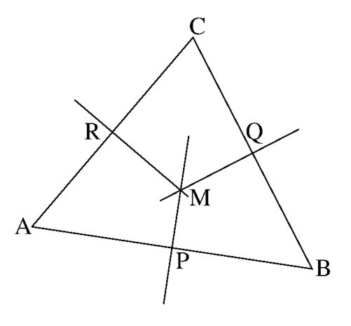
It is well known from planar geometry that the perpendicular medians through
$P$, $Q$ and $R$ have a common intersection point $M$.
The equations of these lines are given by:
\begin{eqnarray*}
\overline{PM} : \quad
& (x,y) = \half (x_A+x_B,y_A+y_B) + \gamma . (y_B-y_A,x_A-x_B) \\
\overline{QM} : \quad
& (x,y) = \half (x_B+x_C,y_B+y_C) + \alpha . (y_C-y_B,x_B-x_C) \\
\overline{RM} : \quad
& (x,y) = \half (x_C+x_A,y_C+y_A) + \beta . (y_A-y_C,x_C-x_A)
\end{eqnarray*}
The intersection point $M$ is associated with values for $\gamma$ , $\alpha$ and
$\beta$, which are labelled as $\gamma_M$ , $\alpha_M$ and $\beta_M$ .
At first $\gamma _M$ and $\alpha _M$ will be calculated, by:
$$
\half (x_A+x_B,y_A+y_B) + \gamma _M . (y_B-y_A,x_A-x_B) =
$$ $$
\half (x_B+x_C,y_B+y_C) + \alpha _M . (y_C-y_B,x_B-x_C)
$$
Giving two equations with two unknowns:
$$
\begin{array}{l}
\half (x_A+x_B) + \gamma _M . (y_B-y_A) =
\half (x_B+x_C) + \alpha _M . (y_C-y_B) \\
\half (y_A+y_B) + \gamma _M . (x_A-x_B) =
\half (y_B+y_C) + \alpha _M . (x_B-x_C)
\end{array} \quad \Longleftrightarrow \quad
$$ $$
\left[ \begin{array}{cc} y_B-y_A & -(y_C-y_B) \\
-(x_B-x_A) & x_C-x_B \end{array} \right]
\left[ \begin{array}{c} \gamma _M \\ \alpha _M \end{array} \right] =
\half \left[ \begin{array}{c} x_C-x_A \\ y_C-y_A \end{array} \right]
$$
The matrix at the left side can be inverted, resulting in:
$$
\left[ \begin{array}{c} \gamma _M \\ \alpha _M \end{array} \right] =
\left[ \begin{array}{cc} x_C-x_B & y_C-y_B \\
x_B-x_A & y_B-y_A \end{array} \right] .
\half \left[ \begin{array}{c} x_C-x_A \\ y_C-y_A \end{array} \right] / \J
$$
Where:
$$
\J = (x_C-x_B)(y_B-y_A)-(x_B-x_A)(y_C-y_B)
$$
Hence:
$$
\gamma _M = \half \left[ (x_C-x_B)(x_C-x_A)+(y_C-y_B)(y_C-y_A) \right] / \J
$$
Define $\vec{r}_{KL} = ( x_L - x_K , y_L - y_K )$ . Then,
with an analogous calculation for $\alpha _M$ and an educated guess for $\beta _M$,
we find:
\begin{eqnarray*}
\gamma _M = \half (\vec{r}_{CA} \cdot \vec{r}_{CB})/ \J \\
\alpha _M = \half (\vec{r}_{AB} \cdot \vec{r}_{AC}) / \J \\
\beta _M = \half (\vec{r}_{BA} \cdot \vec{r}_{BC}) / \J
\end{eqnarray*}
Compare this with our findings in '2-D Resistor Model':
\begin{eqnarray*}
E_{12} = E_{21} = - \half ( \vec{r}_{31} \cdot \vec{r}_{32} )
. \lambda / \J = - 1/R_3 \\
E_{23} = E_{32} = - \half ( \vec{r}_{12} \cdot \vec{r}_{13} )
. \lambda / \J = - 1/R_1 \\
E_{31} = E_{13} = - \half ( \vec{r}_{23} \cdot \vec{r}_{21} )
. \lambda / \J = - 1/R_2
\end{eqnarray*}
With $1 \sim A$ , $2 \sim A$ , $3 \sim C$ , it is concluded that:
$$
\lambda . \gamma _M = 1/R_3 \quad ; \quad
\lambda . \alpha _M = 1/R_1 \quad ; \quad
\lambda . \beta _M = 1/R_2
$$
Assuming that our triangles have non-obtuse angles, we can read from the figure
that $\gamma_M , \alpha_M , \beta_M > 0 $ . In this case:
$$
| \lambda . \gamma_M . (y_B-y_A,x_A-x_B) |
= 1/R_3 . \overline{AB} = \lambda . \overline{PM}
\quad \Longrightarrow \quad
$$ $$
R_3 = \frac{ \overline{AB} }{ \lambda . \overline{PM} } =
\frac{ \mbox{"length" of } R_3 }{ \mbox{conductivity} \, \times \,
\mbox{"diameter" of } R_3 }
$$
In very much the same way we can prove that:
$$
R_1 = \frac{ \overline{BC} }{ \lambda . \overline{QM} } =
\frac{ l_1 }{ \lambda . O_1 } \quad ; \quad
R_2 = \frac{ \overline{CA} }{ \lambda . \overline{RM} } =
\frac{ l_2 }{ \lambda . O_2 }
$$
Where: $ l = $ length, $ O = $ diameter.
This gives us a lucid physical interpretation of the resistances $R_k$, as they
are associated with the linear triangle. It is also seen now why obtuse angles
are more or less unacceptable. In this case one of the resistances will become
negative, meaning that a (heat) current will flow from a place with low
temperature to a place with high temperature, thus violating the Second Law of
Thermodynamics. By "more or less" we mean that any such obtuse angle should be
compensated by a sufficiently sharp one in the opposite triangle, in such a way
that the sum $1/R_a+1/R_b$ of their respective contributions shall be positive.
Having said all this, we would like to generalize the above result, in order to
include Diffusion as well as Convection. An obvious way to do this, is to
make use of the Resistor model, since the latter effectively sets up a link to
the much simpler one-dimensional theory. As follows. When considering
any flux through $\overline{PM}$, the same line segment is associated
with a normal vector $\vec{PM}$ which is perpendicular to it.
Its length is given by:
$$
\overline{PM} =
\gamma_M | (y_B-y_A,x_A-x_B) | = \gamma_M | (x_B-x_A,y_B-y_A) |
= \gamma_M \overline{AB}
$$
This is nice, because $\vec{PM}$ has also the same direction as $\vec{AB}$.
Thus we can put:
$$
\vec{PM} = \gamma_M \vec{AB}
= \half ( \vec{r}_{31} \cdot \vec{r}_{32} ) / \J
\, . \, \vec{r}_{12}
$$
In very much the same way we find:
\begin{eqnarray*}
\vec{QM} = \half ( \vec{r}_{12} \cdot \vec{r}_{13} ) / \J
\, . \, \vec{r}_{23} \\
\vec{RM} = \half ( \vec{r}_{23} \cdot \vec{r}_{21} ) / \J
\, . \, \vec{r}_{31}
\end{eqnarray*}
The Diffusive flux from $(1)$ to $(2)$ through resistor $\overline{AB}$ is:
$$
I^D_{12} = (T_1 - T_2) / R_3 =
\frac{\lambda \overline{PM} }{ \overline{AB} } (T_1 - T_2)
= \half ( \vec{r}_{31} \cdot \vec{r}_{32} ) / \J . \lambda (T_1 - T_2)
$$
Here $(T_1 - T_2)$ is the temperature-difference between $A$ and $B$, $\lambda
= $ thermal conductivity $(J/m/s/K)$.
Analogously, the Convective flux through resistor $\overline{AB}$
is the heat flow coming from $(1)$. It streams through the area $\overline{PM}$
and mixes with the fluid in $(2)$. The net effect is:
$$
I^C_{12} = \rho . c . ( \vec{v} \cdot \vec{PM} ) . (T_1 - T_2)
$$
Here $\rho =$ density $(kg/m^3)$, $c =$ heat capacity $(J/kg/K)$, $\vec{v} =$
velocity $(m/s)$, $T_k =$ local temperature of the fluid $(K)$. Continuing:
$$
I^C_{12} = \rho . c .
\half ( \vec{r}_{31} \cdot \vec{r}_{32} ) / \J .
( \vec{v} \cdot \vec{r}_{12} ) (T_1 - T_2)
$$
So the expressions for Diffusive flux and Convective flux are very much alike:
\begin{eqnarray*}
I^D_{12} = \lambda . G_{12} . (T_1 - T_2) \\
I^C_{12} = \rho . c . ( \vec{v} \cdot \vec{r}_{12} ) . G_{12} . (T_1 - T_2)
\end{eqnarray*}
Where $G_{12} = \half ( \vec{r}_{31} \cdot \vec{r}_{32} ) / \J $ is a purely
geometrical factor, which embodies the geometry of the triangle. The quotient
of Convective and Diffusive flux is entirely independent of that two-dimensional
geometry:
$$
P = \rho . c . ( \vec{v} \cdot \vec{r}_{ij} ) / \lambda
$$
Here $\vec{r}_{ij} = \vec{r}_j - \vec{r}_i = $ vector from $(i)$ to $(j)$. The
projection of the velocity vector on a direction vector replaces the quantity
$\rho.c.v.dx/\lambda$ in the one-dimensional theory. Therefore, $P$ may be
interpreted, again, as a dimensionless local Péclet number.
Now the time has come to generalize a result from Patankar's book
[SV],
namely the formulas (5.47) from 5.2-7 A Generalized Formulation:
\begin{eqnarray*}
&&a_E = D_e A(|P_e|) + \max(-F_e,0) \\
&&a_W = D_w A(|P_w|) + \max(+F_w,0) \\
&&a_P = a_E + a_W + (F_e - F_w)
\end{eqnarray*}
It will be assumed in the sequel that the continuity equation is valid, hence
$F_e - F_w = 0$ . The formulas (5.47) are accompanied with several expressions
for the function $A(|P|)$, as given in
[SV], by Table 5.2 The function
$A(|P|)$ for different schemes:
$$
\begin{array}{ll}
\mbox{Central difference} & A(|P|) = 1 - 0.5 |P| \\
\mbox{Upwind} & A(|P|) = 1 \\
\mbox{Hybrid} & A(|P|) = \max(0,1 - 0.5 |P|) \\
\mbox{Power law} & A(|P|) = \max(0,(1 - 0.1 |P|)^5) \\
\mbox{Exponential (exact)} & A(|P|) = |P|/\left[\exp(|P|)-1\right]
\end{array}
$$
Switching to the Finite Element viewpoint means insisting that assembly of the
F.D. equations shall be done with F.E. matrices, instead of row by row.
Here comes our educated guess of such a matrix:
$$
\left[ \begin{array}{cc} E_{11} & E_{12} \\
E_{21} & E_{22} \end{array} \right] =
\left[ \begin{array}{cc} + a_E & - a_E \\
- a_W & + a_W \end{array} \right]
$$
Since we must be certain that this is indeed the correct matrix, assemble two of
these to a complete equation - which is at the row in the middle - and associate
the proper unknowns:
$$
\left[ \begin{array}{ccc} + a_E & - a_E & 0 \\
- a_W & + a_W + a_E & - a_E \\
0 & - a_W & + a_W \end{array} \right]
\left[ \begin{array}{c} \phi_W \\ \phi_P \\ \phi_E \end{array} \right]
$$
Meanwhile, we have found Linear Triangle equivalents for each of the terms that
constitute $a_E$ and $a_W$:
\begin{eqnarray*}
&&D_{e/w} = G_{ij} \; \lambda\\
&&P_{e/w} = \rho . c . ( \vec{v} \cdot \vec{r}_{ij} ) / \lambda\\
&&F_{e/w} = G_{ij} \; \rho . c . ( \vec{v} \cdot \vec{r}_{ij} )
\end{eqnarray*}
Physical quantities are evaluated at $(e/w)$, corresponding with the middle of
the accompanying resistor elements. A significant detail is the difference
between the $\pm$ signs in:
\begin{eqnarray*}
&&- E_{12} = a_E = D_e A(|P_e|) + \max(- F_e,0) \\
&&- E_{21} = a_W = D_w A(|P_w|) + \max(+ F_w,0)
\end{eqnarray*}
No reason to bother, however, because when evaluated at the same place:
$$
+ F_w = \rho . c . ( \vec{v} \cdot \vec{r}_{12} ) =
- \rho . c . ( \vec{v} \cdot \vec{r}_{21} ) \hieruit
- E_{ij} = D_{ij} A(|P_{ij}|) + \max(- F_{ij} ,0)
$$
Further simplification will be achieved by assuming that $\lambda$ is a constant
and dividing the quantities $D_{e/w} = D_{ij}$ and $F_{e/w} = F_{ij}$ by this
conductivity:
\begin{eqnarray*}
&&D_{ij} / \lambda = G_{ij} \\
&&P_{ij} = \rho . c . ( \vec{v} \cdot \vec{r}_{ij} ) / \lambda\\
&&F_{ij} / \lambda = G_{ij} \; P_{ij}
\end{eqnarray*}
The end result is an F.E. matrix which is suitable for Convection And Diffusion:
$$
\left[ \begin{array}{cc} + E_{12} & - E_{12} \\
- E_{21} & + E_{21} \end{array} \right]
\qquad \mbox{where:} \qquad
E_{ij} = G_{ij} \; \left[ A(|P_{ij}|) \, + \, \max(0, - P_{ij}) \right]
$$
It is remarked that the above generalization is faithful, meaning that it
is reduced exactly to Patankar's original scheme, when specialized for a
rectangular grid. (Such a thing is not accomplished, strangely enough, with the
F.E. formulation as devised by Patankar himself in
[SV], paragraph 8.4-3).
Our theory is accompanied with a sample program, which has been coded in Delphi
Pascal. Heat Transfer is described there by the following PDE:
$$
P\!e \left[ u \dq{T}{x} + v \dq{T}{y} \right]
- \left[ \dq{^2 T}{x^2} + \dq{^2 T}{y^2} \right] = 0
$$
$P\!e =$ overall Péclet number, $(x,y) =$ normed coordinates, $(u,v) =$ normed
velocity field, $T = $ temperature.
My favorite sample flow field is given by the conformal (complex) mapping
$ \zeta = z^2/2 $. Taking the real and the complex part of it gives rise to a
potential function $\phi$ and a stream function $\psi$ respectively:
$$
\phi(x,y) = \half (x^2 - y^2) \EN \psi(x,y) = x.y
$$
Contours of the functions $\phi$ and $\psi$ form two systems of orthogonal
hyperbolas.
These hyperbolas are mutually orthogonal where they intersect. The points of
intersection form the basis of a triangular mesh. They are found as follows:
$$
\half ( x^2 - y^2) = A \EN x.y = B \hieruit \half x^2 - \half (B/x)^2 = A
$$ $$
\hieruit x^4 - 2 A x^2 - B^2 = 0 \hieruit x^2 = \sqrt{A^2 + B^2} \pm |A|
$$ $$
\hieruit x = \sqrt{\sqrt{A^2 + B^2} \pm |A|} \EN y = \sqrt{x^2 - 2 A}
$$
The domain of interest is bounded by x-axis, y-axis and relevant outer pieces
of the hyperbolas. The velocity field is derived from either the potential or
the stream function:
$$
u = \dq{\phi}{x} = \dq{\psi}{y} = x
\EN v = \dq{\phi}{y} = - \dq{\psi}{x} = - y
$$
Our theory seems to be finished herewith. The rest is a matter of technology.