Conservation of Heat
$
\def \half {\frac{1}{2}}
\def \kwart {\frac{1}{4}}
\newcommand{\dq}[2]{\displaystyle \frac{\partial #1}{\partial #2}}
\newcommand{\oq}[2]{\partial #1 / \partial #2}
\def \J {\Delta}
$
The Numerical Analysis of Diffusion starts with a well known Partial
Differential
Equation (PDE). The problem will be restricted here to the simpler case of
two space dimensions:
$$
\dq{Q_x}{x} + \dq{Q_y}{y} = 0
$$
$ (x,y) = $ Planar coordinates. A possible interpretation of the vector
$ (Q_x,Q_y) $ is the heat flux. The differential equation then follows from the
law of conservation of energy. In case of pure diffusion of heat, also known
as conduction, the components of the heat flux are related to temperature as
follows:
$$
Q_x = - \lambda \dq{T}{x} \qquad \qquad Q_y = - \lambda \dq{T}{y}
$$
Where $ \lambda = $ thermal conductivity. Hence the final differential equation
for the temperature field is actually of the second degree. In order to make
the PDE amenable for numerical treatment, an integration procedure has to be
resorted to. At this point, there occurs a splitting into several distinct
roads, all leading to a numerical solution, more or less efficiently.
When using a Finite Element method, the differential equation is multiplied at
first with an arbitrary (test)function. Subsequently the PDE is integrated over
the domain of interest. Let the test function be called $f$, then:
$$
\iint f . \left[ \dq{Q_x}{x} + \dq{Q_y}{y} \right] \, dx dy = 0
$$
It can be shown that this integral formulation is equivalent with the original
partial differential equation. This is due to the fact that $f$ is an
arbitrary function. It should be continuous and integrable, though.
Partial integration, or applying Green's theorem (which is precisely the same),
results in an expression with line-integrals over the boundaries and an area
integral over the bulk field. The latter is given by:
$$
- \iint \left[ \dq{f}{x}.Q_x + \dq{f}{y}.Q_y \right] \, dx dy
$$
Watch the minus sign. The advantage accomplished herewith is a reduction of the
difficulty of the problem: only derivatives of the first degree are left.
As a next step, the domain of interest is split up into "elements" $E$.
Due to this, also the integral will split up into separate contributions,
each contribution corresponding with an element:
$$
- \sum_E \iint \left[ \dq{f}{x}.Q_x + \dq{f}{y}.Q_y \right] \, dx dy
$$
The simplest Finite Element in two dimensions is the linear triangle: read the
previous section titled "Triangle Algebra". Essential ingredient of the theory
is the so called Differentiation Matrix. Any partial derivative at a linear
triangle can be discretized easily with help of such a differentiation matrix:
$$
\J \left[ \begin{array}{c} \oq{f}{x} \\ \oq{f}{y} \end{array} \right] =
\left[ \begin{array}{ccc} +(y_2 - y_3) & +(y_3 - y_1) & +(y_1 - y_2) \\
-(x_2 - x_3) & -(x_3 - x_1) & -(x_1 - x_2) \end{array}
\right] \left[ \begin{array}{c} f_1 \\ f_2 \\ f_3 \end{array} \right]
$$
Here $\J$ is the area of a vector parallelogram, which is twice the area of the
triangle.
It is clear that $\oq{f}{x}$ and $\oq{f}{y}$ are constants. While considering
only 2-D diffusion, $Q_x$ and $Q_y$ are also partial derivatives of the first
degree, hence constants. Herewith the bulk Finite Element formulation, for one
triangle, is given by:
$$
- \left[ \dq{f}{x}.Q_x + \dq{f}{y}.Q_y \right] \iint dx dy =
- \left[ \dq{f}{x}.Q_x + \dq{f}{y}.Q_y \right] \J/2
$$
The remaining integral is equal, namely, to de area of the triangle. Applying now
the differentiation matrix, we find:
$$
= - \half \left[ \begin{array}{ccc} f_1 & f_2 & f_3 \end{array} \right]
\left[ \begin{array}{cc} y_2 - y_3 & x_3 - x_2 \\
y_3 - y_1 & x_1 - x_3 \\
y_1 - y_2 & x_2 - x_1 \end{array} \right]
\left[ \begin{array}{c} Q_x \\ Q_y \end{array} \right] =
$$ $$
= \half \left[ \begin{array}{ccc} f_1 & f_2 & f_3 \end{array} \right]
\left[ \begin{array}{c} (y_3 - y_2) Q_x - (x_3 - x_2) Q_y \\
(y_1 - y_3) Q_x - (x_1 - x_3) Q_y \\
(y_2 - y_1) Q_x - (x_2 - x_1) Q_y \end{array} \right]
$$
Actually, we don't want to subdivide the Finite Element domain into triangular
elements, but rather into quadrilateral elements. However, any quad element,
in turn, can be subdivided yet into triangles, even in two different ways:
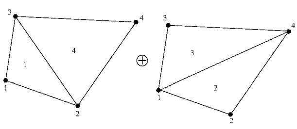
In addition, what we want is a configuration in which all quad vertices play an
equally important role. In order to accomplish this, all of the four triangles
must be present in our formulation, simultaneously. For just one quadrilateral,
it boils down to renumbering vertices in the formulation for a single triangle,
according to the following permutations:
1 2 3 2 4 1 3 1 4 4 3 2
Also an upper label (not a power) will be attached to the values $(Q_x,Q_y)$,
because it must be denoted at which triangle the discretization takes place.
Any contributions are summed now over the four triangles (and the whole is divided
by a factor two again):
$$
\kwart \left[ \begin{array}{ccc} f_1 & f_2 & f_3 \end{array} \right]
\left[ \begin{array}{c} (y_3 - y_2) Q^1_x - (x_3 - x_2) Q^1_y \\
(y_1 - y_3) Q^1_x - (x_1 - x_3) Q^1_y \\
(y_2 - y_1) Q^1_x - (x_2 - x_1) Q^1_y
\end{array} \right] +
$$ $$
\kwart \left[ \begin{array}{ccc} f_2 & f_4 & f_1 \end{array} \right]
\left[ \begin{array}{c} (y_1 - y_4) Q^2_x - (x_1 - x_4) Q^2_y \\
(y_2 - y_1) Q^2_x - (x_2 - x_1) Q^2_y \\
(y_4 - y_2) Q^2_x - (x_4 - x_2) Q^2_y
\end{array} \right] +
$$ $$
\kwart \left[ \begin{array}{ccc} f_3 & f_1 & f_4 \end{array} \right]
\left[ \begin{array}{c} (y_4 - y_1) Q^3_x - (x_4 - x_1) Q^3_y \\
(y_3 - y_4) Q^3_x - (x_3 - x_4) Q^3_y \\
(y_1 - y_3) Q^3_x - (x_1 - x_3) Q^3_y
\end{array} \right] +
$$ $$
\kwart \left[ \begin{array}{ccc} f_4 & f_3 & f_2 \end{array} \right]
\left[ \begin{array}{c} (y_2 - y_3) Q^4_x - (x_2 - x_3) Q^4_y \\
(y_4 - y_2) Q^4_x - (x_4 - x_2) Q^4_y \\
(y_3 - y_4) Q^4_x - (x_3 - x_4) Q^4_y
\end{array} \right] \mbox{ }
$$
Another way to arrive at a formulation in which all
four triangles are involved is via Numerical Integration. The implementation of
numerical integration is done most efficiently, for quadrilaterals, by choosing
four integration points (often called Gauss points) inside the quadrilateral.
According to standard theory, these points are located at positions $(\xi,\eta)
= 1/(2\sqrt{3})$. (Read the section "Quadrilateral Algebra" for an explanation
of $\xi$ and $\eta$). It is possible, however, to interpret the exact location
of the "Gauss" points with a pinch of salt. The integration points then can be
located simply at the vertices (which are only a small distance apart from the
"true" locations anyway). Quadrilaterals then behave as if they are composed of
overlapping triangles, as depicted in the above figure. It is also clearer now
where the weighting factor $1/4$ comes from: there are $4$ integration points.
And quantities $Q^k$ are associated not only with the four triangles, but also
with the four vertices of the original quadrilateral.
In order to save unnecessary paperwork, the following shorthand notation has
been adopted. It may be interpreted as an outer product:
$$
r_{ij} \times Q_k = (y_i - y_j) Q^k_x - (x_i - x_j) Q^k_y
= (x_j - x_i) Q^k_y - (y_j - y_i) Q^k_x
$$
Terms belonging to $f_k, k=1 ... 4$ are collected together. By doing so, the
standard Finite Element assembly procedure is demonstrated at a small scale.
What else is the Finite Element matrix than just an incomplete system of
equations?
$$
\kwart \left[ \begin{array}{cccc} f_1 & f_2 & f_3 & f_4 \end{array} \right]
\left[ \begin{array}{c}
r_{32} \times Q_1 + r_{42} \times Q_2 + r_{34} \times Q_3 + 0 \\
r_{13} \times Q_1 + r_{14} \times Q_2 + 0 + r_{34} \times Q_4 \\
r_{21} \times Q_1 + 0 + r_{41} \times Q_3 + r_{42} \times Q_4 \\
0 + r_{21} \times Q_2 + r_{13} \times Q_3 + r_{23} \times Q_4
\end{array} \right]
$$
Subsequently use:
$$
r_{32} = r_{34} + r_{42} \qquad r_{14} = r_{13} + r_{34} \qquad
r_{41} = r_{42} + r_{21} \qquad r_{23} = r_{21} + r_{13}
$$
To put the above in a more handsome form:
$$
\left[ \begin{array}{cccc} f_1 & f_2 & f_3 & f_4 \end{array} \right]
\left[ \begin{array}{c}
\half r_{42} \times \half (Q_1+Q_2) + \half r_{34} \times \half (Q_1+Q_3) \\
\half r_{13} \times \half (Q_1+Q_2) + \half r_{34} \times \half (Q_2+Q_4) \\
\half r_{21} \times \half (Q_1+Q_3) + \half r_{42} \times \half (Q_3+Q_4) \\
\half r_{21} \times \half (Q_2+Q_4) + \half r_{13} \times \half (Q_3+Q_4)
\end{array} \right]
$$
It's a triviality, but nevertheless: a picture says more that a thousand words.
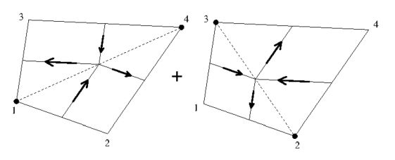
It is seen that the four pieces-of-equations correspond with four pieces of
line-integrals, each of them belonging to one of the vertices. Midpoints of
triangle sides are connected by lines at which the integration takes place.
The heat flux at a midpoint is the average of values at the vertices.
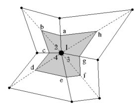
Let's adopt another point of view now and no longer concentrate on elements but
on vertices. Instead of arranging vertices around an element, elements are
arranged around a vertex. Label triangle side midpoints as $a,b,c,d,e,f,g,h$.
It is immediately noted that the lines connecting the midsides of the triangles
around a vertex, when tied together, neatly delineate a closed area, which can
be interpreted as a kind of 2-D Finite Volume. Expressed in the outer product
formalism, we find:
$$
r_{ba} \times Q_a + r_{cb} \times Q_c + r_{dc} \times Q_c +
r_{ed} \times Q_e + r_{fe} \times Q_e + r_{gf} \times Q_g +
r_{hg} \times Q_g + r_{ah} \times Q_a
$$
Which is the content of one equation in the Finite Element global matrix.
All terms together represent a discretization of the following circular
integral:
$$
\sum r \times Q = \oint Q_y dx - Q_x dy
$$
With help of Green's theorem, however, such a circular integral can be converted
into a "volume" integral, over the area indicated in the above figure:
$$
\oint Q_y dx - Q_x dy =
+ \iint \left[ \dq{Q_x}{x} + \dq{Q_y}{y} \right] \, dx dy
$$
Conservation of heat is integrated over a finite volume, which is wrapped around
a vertex. So we have arrived at a Finite Difference method. To be more precise:
at a Finite Volume method. It is remarked that this F.V. procedure has been
applicable for curvilinear grids from the start.
Thus we derived a Theorem which Unifies a Finite Element and a Finite
Volume method, for a rather general class of 2-D diffusion problems:
Apply a Finite Element (Galerkin) method to a mesh of quadrilaterals. Subdivide
each of the quads into four (overlapping) triangles, in the two ways which are
possible. Then such a method is {\bf equivalent} to a Finite Volume method:
midsides of the triangles, around the vertex of interest, are neatly connected
together, to form the boundary of a 2-D finite volume, and the conservation law
is integrated over this volume.
A Unification Theorem like the above may have a couple of practical consequences,
as will be investigated in the sequel.