Critical Mass Flow

Even more crude than the ideal flow assumption, but - as we shall see - not very different from it, is the following point of view, which shall be called the TA/K model for historical reasons. People have had in mind the following picture of the shell side flow, at the outlet of the tube bundle for example:

Consider a ring shaped element in the liquid at the outflow area. The inner radius of this element is equal to the (outer) radius $R$ of the central tube. The outer radius of the ring is called $r$ and is a variable. The height of the ring is equal to the height $F$ of the outflow perforation. The back side of the ring (central tube) as well as the bottom (tube plate) are solid material. Therefore the flux through the upper side must always be equal to the flux through the front side. For the sake of simplicity it is assumed that the medium streams into the ring with a constant mid-bundle velocity, which may be normed to $1$. The velocity component $u$ can now be calculated from: $$ \pi.(r^2 - R^2).1 = 2.\pi.r.F.u \qquad \Longrightarrow \qquad u = \frac{r^2 - R^2}{2.F.r} = \frac{1}{2.F} \left( r - \frac{R^2}{r} \right) $$ Thus the total mass flow coming in from the bundle is balanced with the mass flow going out through the outflow perforation. We will demonstrate now that this primitive picture of the flow field does correspond anyway with ideal flow. Assume for the component $v$ that it is linear with $z$ in the axial direction, which is the simplest possible assumption. The other component $u$ is already known: $$ v = - \frac{z}{F} \qquad ; \qquad u = \frac{ r^2 - R^2}{2.F.r} $$ It can be checked out easily that this field $(u(r),v(z))$ is indeed a solution of the partial differential equations describing ideal flow in a cylindrically symmetric geometry. Yet there is a small flaw in this reasoning. At the upper side of the perforation $F$, namely, the vertical component $v$ becomes $-1$, the mid-bundle velocity, as it should. However, the horizontal component $u$ suddenly becomes zero ! Giving rise to a kink in the streamlines, which is physically impossible, of course. Nevertheless, when considered as a crude first approximation, the TA/K model is not so bad after all. So far so good for the flow field.

Let's proceed with the equations for Heat Transfer in the fluid tube continuum, as they have been presented in the previous section.
To begin with, the heat transfer equations can be integrated exactly at the less interesting part of the tube bundle, where the flow streams parallel to the tubes and thus is no longer two-dimensional. For that mid-bundle area, a so-called one-tube model can be employed, which turns out to be a system of two coupled ordinary differential equations. Such a system can be solved by standard means. There is nothing new here.
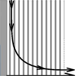
But, apart from the parallel flow area, analytical solutions can be found for some other places in the heat exchanger. Such a solution can be constructed rather easily for a streamline which runs from the join between the central tube and the lower tube plate towards the outflow perforation:

The equations there reduce to an ordinary differential equation for primary temperatures, because the secondary temperature is a boundary condition. In addition, we have an expression for the flow distribution in place, according to the TA/K model. Substitution of the latter into the Heat Transfer equation for the Primary medium leads to: $$ c.G_P.\frac{1}{2.F} \left( r - \frac{R^2}{r} \right) \frac{dT_P}{dr} + a.[ \, T_P - T_{S0} \, ] = 0 $$ The solution of such an ordinary differential equation is routinely found with Operator Calculus: $$ \left[ \frac{d}{dr} + \frac{2.r.F.a/(c.G_P)}{r^2 - R^2} \right] (T_P - T_{S0}) = 0 $$ The following term must be integrated: $$ \int \frac{2.r.F.a/(c.G_P)}{r^2 - R^2} \, dr = \frac{F.a}{c.G_P} \int \frac{dr^2}{r^2 - R^2} = \frac{F.a}{c.G_P} \ln \left( \frac{r^2}{R^2} -1 \right) $$ Herewith, the differential equation is transformed into: $$ \left( \frac{r^2}{R^2} -1 \right)^{ - F.a/(c.G_P) } \: \frac{d}{dr} \: \left( \frac{r^2}{R^2} -1 \right)^{ + F.a/(c.G_P) } \: (T_P - T_{S0})= 0 $$ And the solution of it is: $$ T_P - T_{S0} = K.\left( \frac{r^2}{R^2} -1 \right)^{ - H } \quad \mbox{where} \quad H = F.a/(c.G_P) $$ Furthermore, $K$ is a (rather) unknown constant. Because $(r^2/R^2 - 1)$ becomes zero in the corner for $r=0$ and the quantity $-H$ is a negative power, it must be concluded that the solution is singular. Well, of course not ! Infinities of this nature cannot exist, at all, in a heat exchanger.

There are no black holes in a simple chemical apparatus. On physical grounds, we can be absolutely certain that all temperatures are in between the following bounds: $T_{S0}$, the secondary inlet-temperature and $T_{PL}$, the primary inlet-temperature. Therefore we must conclude that the constant $K$ can be nothing else but zero. As a consequence herefrom, along the streamline at the bottom of the apparatus: $T_P = T_{S0}$. Meaning that the primary temperature is equal to the secondary inlet-temperature everywhere at the lower tube plate.
But now it seems that we have gone a bit too far. To refresh our memory, the fluid tube continuum model is meant to be a crude model of a discrete reality. Therefore we should always put question marks at the validity of the model. Especially, attention is required as soon as singularities become apparent in the model. Spots at which singularities occur are suspect without question. Infinities cannot physically exist anyway. But instead of assigning immediately the null-solution, we should think of another possibility. A singularity can also be a signal that our continuum hypothesis is no longer a valid assumption, for certain spots in the model. 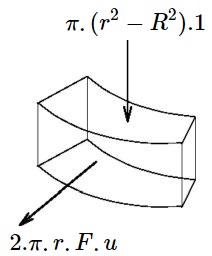It is clear that, with the fluid tube continuum model, the solution is an approximation only for infinitesimal volumes with a size greater than the pitch between tubes. If we smear out the solution over a ring with size $s$ (of the pitch), then it should approximately be the same solution again. Let this be exemplified for our abovementioned analytical solution (where it is assumed for convenience that $H \neq 1$): $$ K.\frac{ \int_{x}^{x+s} \left[ \, (r/R)^2-1 \, \right]^{-H} \, 2.\pi.r.dr }{ \pi.[ \, (x+s)^2 - x^2 \, ] } = $$ $$ \frac{K}{1-H}. \frac{ \left[ \left( \frac{x+s}{R} \right)^2 - 1 \right]^{1 - H} - \left[ \left( \frac{x}{R} \right)^2 - 1 \right]^{1 - H} } { \left( \frac{x+s}{R} \right)^2 - \left( \frac{x}{R} \right)^2 } $$ Here $s=$ the pitch of the tube bundle; $H = F.a/(c.G_P)$. Quite another picture is emerging now. The singularity becomes weakened by smearing it out over the pitch. Two distinct cases can be distinguished:

$H > 1 $ . Still a true singularity.
The conclusions about the null-solution remain valid: $T_P = T_{S0}$.
$H < 1 $ . The singularity doesn't exist anymore.
Conclusions about the null-solution are likely to be invalid. The primary temperature doesn't become coincident with the secondary temperature everywhere: $T_P \neq T_{S0}$.

The condition $\,H < 1\,$ means that $\,F.a/c.G_P < 1\,$ or $\,G_P > F.a/c$ . The physical meaning of the latter is that the primary mass flow is so large that the heat contained in it can not be transferred over a height $\,F\,$ within the distance $\,s$ , which is the pitch between the tubes. But this in turn means that one of the basic conditions of the continuum model is no longer valid. The "differential" $\,s\,$ between the tubes becomes sensible, so to speak. The primary medium is not "really" continuous anymore. The discrete substrate, the fine structure of the bundle is no longer "invisible". We could call the value $\,G_P\,$, where $\,G_P = F.a/c$ , a critical mass flow. It is the mass flow where the Continuum breaks down to the Discrete, so to speak.

It is a nice exercise to actually calculate this critical mass flow for a real world heat exchanger, which happens to be the Neratoom IHX (Intermediate Heat Exchanger). The IHX was meant to operate in the hot leg of a Liquid Metal Fast Breeder Reactor (LMFBR), namely SNR-300 in Kalkar, West-Germany.

  program test;

  function critical : double;
  const
    NP : double = 846 ; { number of tubes }
    DO : double = 0.0210 ; { outer diameter of tubes }
    DI : double = 0.0182 ; { inner diameter of tubes }
    L : double = 20 ; { conductivity of tube walls }
    F : double = 0.370 ; { height of outflow perforation }
    C : double = 1275; { heat capacity of sodium }
  var
    A : double; { heat transfer coefficient }
  begin
    A := NP*2*Pi*L/ln(DO/DI);
    critical := F*A/C;
  end;

  begin
    Writeln(critical:4:1,' kg/s');
  end.

The outcome is : $G_P = 215.6 \, kg/s$ . The fine structure of the IHX tube bundle may have been observable, since large scale physical experiments , with primary mass flows varying between $80$ and $360 \, kg/s$, have been actually carried out in a test facility. And our calculated value of the critical mass flow is clearly in that range. Thus the discrete substrate of the fluid tube continuum could have been visible as such.
Should it be concluded, more generally, that singularities, where they cannot occur physically - question: can they ever occur physically ? - are just a signal that some continuum model is no longer valid at some place ?