With the 2-D Navier-Stokes equations for incompressible & stationary flow, there is an abundance of more or less proper boundary conditions in literature. Some of these are incredibly complicated, so I'd suggest to hunt for the simple ones. More or less by coincidence, I've stumbled upon a decent example for duct flow:
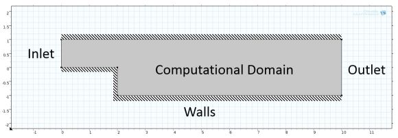
The acccompanying picture illustrating the boundary conditions is resemblant to the OP's:
Then the article says: The fluid velocity is specified at the inlet and pressure prescribed at the outlet.
A no-slip boundary condition (i.e., the velocity is set to zero) is specified at the walls.
This means that, at the inlet area, the full velocity vector field must be specified: $(u_i,v_i) = (U,V)$.
If there is no reason to assume otherwise, then an uniform velocity field may be imposed.
The pressure condition at the outlet area comes as a slight surprise for me, but I think it's more reasonable
than trying to impose a velocity field. The reason is that you will get in trouble while trying to fulfull
the global conservation laws for mass and momentum. An extreme example is the outlet velocity field
$(u_o,v_o) = (0,0)$ that will suck all mass into nothingness; I can only hope that the CFD code will protest
against this, but have the sad experience that too often it will not.
If there is no reason to assume otherwise,
then an uniform pressure field may be imposed.
Last but not least, the no-slip boundary conditions are commonly assumed to be correct.
If is is assumed in addition that the flow is irrotational, then the no-slip boundary conditions
must be replaced by impermeability conditions, of the form $\;(u,v) \cdot (n_{wx},n_{wy}) = 0$ .
The boundary conditions as proposed by the OP for the inlet area are entirely correct
for such ideal / potential flow, as it is called : $(u,v) \cdot (n_{ix},n_{iy}) = $ given.
Boundary conditions for the outlet area are: velocities parallel to the normal $\,(u,v)\, //\, (n_{ox},n_{oy})$ .
Then let the CFD code be good enough to assure that e.g. global mass conservation is guaranteed.
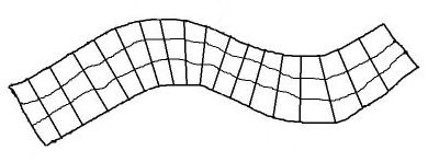
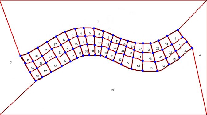
This is pattern recognition ? Yes it is ! Now we can generate the final (neat) finite element mesh for the purpose of making calculations:
This is very much resemblant to the Finite Difference / Finite Volume / Finite Element mesh in the abovementioned
key reference,
which is no coincidence of course.
See the last part of my
previous answer
for (a possible choice of) the boundary conditions.
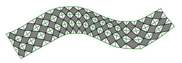
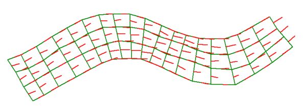
Here comes an impression of the velocity field
as calculated with Ideal Internal Flow and our (Least Squares)
Unified Numerical Analysis:
Last but not least, the software (Delphi Pascal source code) @
MSE publications / references 2017 .