As the OP says, Wikipedia has a wild article about the Dirac delta "function". Interestingly enough, I think that there are a few good things in that wild article. The first good thing is the picture right on top:

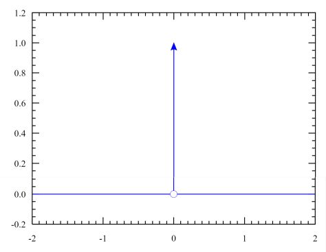
It may be a problem analytically, but when seen from a purely geometrical viewpoint, there is no problem at all: the Dirac delta is the union of the $x$ - axis and the positive part of the $y$ - axis. More precisely, it is the set $$ \{(x,y)\in\mathbb{R}^2|((y=0)\land(x\ne 0))\lor((x=0)\land(y>0))\} $$ Apart from the fact that (half)lines in Euclidean geometry cannot have an area, while the Dirac delta has one $=1$.

It's typical that the Dutch Diracdelta Wikipedia has an aditional section about Approximations with test functions. There are two nice GIF animations in the article showing how it works,

• with a Gauss function : $\large \delta_\sigma(x) = \frac{1}{\sigma\sqrt{2\pi}}e^{-(x/\sigma)^2/2}$
• with a Sinc function : $\large \delta_\sigma(x) = \frac{\sin(x/\sigma)}{\pi.x} = \frac{\sin(x/\sigma)}{\sigma.\pi.(x/\sigma)}$

Dirac Delta Test Functions

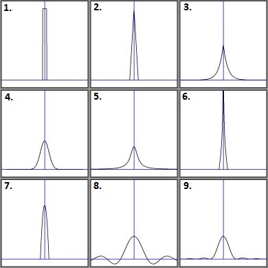
The secret is in scaling (with $\sigma$). Let $T(x)$ be one of the Test functions. Then quite in general we have, for any approximation of the Dirac delta with such a Test function ($\sigma > 0$) : $$ \delta_\sigma(x) = \frac{1}{\sigma}T\left(\frac{x}{\sigma}\right) \\ \int_{-\infty}^{+\infty}\delta_\sigma(x)\, dx = \int_{-\infty}^{+\infty} T\left(\frac{x}{\sigma}\right) d\left(\frac{x}{\sigma}\right) = \int_{-\infty}^{+\infty} T(x)\, dx = 1 $$ According to a sloppy definition, maybe used by some physicists, we have: $$ \delta(x) = \lim_{\sigma\to 0} \delta_\sigma(x) = \lim_{\sigma\to 0} \left[\frac{1}{\sigma}T\left(\frac{x}{\sigma}\right)\right] = 0 \quad \mbox{for} \quad x \ne 0 $$ Sloppy because, upon inspection, this limit covers only part of the geometrical representation, namely: $$ \{(x,y)|(y=0)\land(x\ne 0)\} \quad \mbox{but not} \quad \{(x,y)|(x=0)\land(y>0)\} $$ In order to cover the half $y$-axis case, we might need the inverse of the test function: $$ y = \frac{1}{\sigma}T\left(\frac{x}{\sigma}\right) \quad \Longrightarrow \quad x = \sigma.T^{-1}(y.\sigma) $$ And another limit, expressing that the upper $y$ - axis is approximated as closely as we want: $$ \lim_{\sigma\to 0} \left[\sigma.T^{-1}(y.\sigma)\right] = 0 $$ Example. Take test function number (5.), which is the Cauchy distribution: $$ T(x) = \frac{1/\pi}{1+x^2} \quad \Longrightarrow \quad \delta_\sigma(x) = \frac{1}{\sigma}T\left(\frac{x}{\sigma}\right) = \frac{1/(\pi\sigma)}{1+(x/\sigma)^2} $$ The inverse function (two branches) is found in a few steps: $$ y = \frac{1/(\pi\sigma)}{1+(x/\sigma)^2} \\ \frac{1}{\pi\sigma.y} = 1+(x/\sigma)^2 \\ x = \pm\sigma\sqrt{\frac{1}{\pi\sigma.y}-1} $$ For the sake of completeness: $$ \delta_\sigma^{-1}(y>0) = \begin{cases} \pm\sigma\sqrt{1/(\pi\sigma.y)-1} & \mbox{for} & y \le 1/(\pi\sigma) \\ 0 & \mbox{for} & y > 1/(\pi\sigma) \end{cases} $$ It is clear that for $x\ne 0$ : $$ \lim_{\sigma\to 0} \delta_\sigma(x) = \lim_{\sigma\to 0} \frac{1/(\pi\sigma)}{1+(x/\sigma)^2} = \frac{\sigma/\pi}{\sigma^2+x^2} = 0 $$ On the other hand, for $\,0 < y \le 1/(\pi\sigma)$ : $$ \lim_{\sigma\to 0} \delta^{-1}_\sigma(y) = \lim_{\sigma\to 0} \pm\sigma\sqrt{\frac{1}{\pi\sigma.y}-1} = \lim_{\sigma\to 0} \pm\sqrt{\frac{\sigma}{\pi.y}-\sigma^2} = 0 $$ Thus, in the limit, the Dirac delta is indeed equal to the geometry that is represented by the set $\{(x,y)\in\mathbb{R}^2|((y=0)\land(x\ne 0))\lor((x=0)\land(y>0))\}$ .