Persistent Properties

$ \def \half {\frac{1}{2}} \def \EN {\quad \mbox{and} \quad} \def \slechts {\quad \Longleftrightarrow \quad} \def \hieruit {\quad \Longrightarrow \quad} $ Suppose we have a uniform grid and let $j > i$. Then all coefficients $a_{ij}$ may be assumed to be equal to each other. The same is true for all coefficients $a_{ji}$. Let $a_{ij}=-a$ and $a_{ji}=-b$. Also assume that the system matrix $S$ has been (re)normalized. Then the general form of such a matrix is: $$ \left[ \begin{array}{ccccccc} . & . & . & & & & \\ & -b & 1 & -a & & & \\ & & -b & 1 & -a & & \\ & & & -b & 1 & -a & \\ & & & & . & . & . \end{array} \right] = S = I - M $$ The matrix $M^2$ is calculated: $$ \left[ \begin{array}{ccccccc} . & . & . & & & & \\ & b^2 & 2.a.b & a^2 & & & \\ & & b^2 & 2.a.b & a^2 & & \\ & & & b^2 & 2.a.b & a^2 & \\ & & & & . & . & . 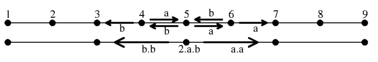\end{array} \right] = M^2 $$ It is seen that, at a coarser grid, the coefficients are obtained by travelling two steps in any direction on the refined grid, multiplying the accompanying matrix-coefficients with each other and adding together the results of each of the possible paths. (This vaguely reminds to a piece of QuantumElectroDynamics.) Hence, travelling from (5) to (4) gives a contribution $b.b$, travelling from (5) to (7) gives a contribution $a.a$ and travelling from (5) to (5) two times back and forth gives a contribution $a.b + b.a$:

Completing further one step of the Newton-Raphson procedure results in: $$ \left[ \begin{array}{ccccccc} . & . & . & & & & \\ & -b^2 & 1-2.a.b & -a^2 & & & \\ & & -b^2 & 1-2.a.b & -a^2 & & \\ & & & -b^2 & 1-2.a.b & -a^2 & \\ & & & & . & . & . \end{array} \right] = I - M^2 = S' $$ Where $S'$ is a blocked matrix, corresponding with 2 coarser grids. Now it is sensible to require that $(I - M^2)$, after re-normalization, has properties which are more or less alike those of $(I - M)$. Essentially the same kind of discretization scheme should be used at any of the coarser or refined grids. It's useful to give a name to the phenomenon. If certain properties of a scheme remain the same at any of the MultiGrids, then such Properties will be called Persistent.
After renormalization, the off-diagonal coefficients become: $$ a' = \frac{a^2}{1-2.a.b} \EN b' = \frac{b^2}{1-2.a.b} $$ Under the obvious assumption that $1 - 2.a.b \ne 0$.
And we are ready to find our first persistent properties, though maybe they are somewhat trivial: $$ a = 0 \slechts a' = 0 \qquad \EN \qquad b = 0 \slechts b' = 0 $$ So far so good. Let's consider cases where $a \ne 0$ and $b \ne 0$. From the coarsening formulas for $a$ and $b$, it can then be inferred immediately that: $$ \frac{a'}{b'} = \frac{a^2}{b^2} > 0 $$ While multiplying $a'$ and $b'$ gives: $$ a'.b'= \frac{a^2.b^2}{(1-2.a.b)^2} > 0 $$ Four different cases may be distinguished: \begin{eqnarray*} a > 0 \EN b < 0 & \qquad & a < 0 \EN b > 0 \\ a < 0 \EN b < 0 & \qquad & a > 0 \EN b > 0 \end{eqnarray*} The formulas for the quotient and the product show that only a positive product and a positive quotient of the off-diagonal coefficients can be actually persistent through coarser multigrids. Hence combinations $a > 0 , b < 0$ and $a < 0 , b > 0$ are already out of the question. Thus, the only properties which may be invariant for grid coarsening are: both coefficients negative or both coefficients positive. We are ready now to infer one of the inverse functions, which is applicable to grid refinement instead of grid coarsening: $$ \frac{a'}{b'} = \frac{a^2}{b^2} \slechts \frac{a}{b} = \sqrt{\frac{a'}{b'}} $$ Substituting $a=\sqrt{a'/b'}.b$ into $b'=b^2/(1-2.a.b)$ leads to an equation from which $b$ can be solved: $$ b' = b^2/(1 - 2.a.b) \hieruit b' - 2.a.b.b' = b^2 \hieruit b' - 2.\sqrt{a'/b'}.b.b.b' = b^2 $$ $$ \hieruit b' = 2.\sqrt{a'.b'}.b^2 + b^2 \hieruit b' = b^2.(1 + 2.\sqrt{a'.b'}) > 0 $$ Almost the same can be done for $a$: $$ a' = a^2.(1 + 2.\sqrt{a'.b'}) > 0 $$ Herewith also the condition $a<0 , b<0$ is ruled out as a possible persistent property, leaving $a>0 , b>0$ as the only possibility left. We conclude that the following is a necessary condition for persistence, given $-a$ and $-b$ as the off-diagonal elements in a (normed) tri-diagonal system, while admitting again the special cases $a = 0$ and/or $b = 0$: $$ a \ge 0 \EN b \ge 0 $$ The well known and commonly accepted "rule of positive coefficients" (Patankar 1980) is found back herewith.
The inverse of mesh coarsening, grid refinement, seems to be at least equally important as the former. Given the discretization on a coarser grid, how can we obtain then the discretization on a finer grid? It is clear that grid refinement, in general, can be quite ambiguous. That's one reason why, probably, we shall have to restrict ourselves to uniform grids.
Inverse functions can be derived for the off-diagonal coefficients as such: $$ a' = a^2/(1 - 2.a.b) \slechts a = \sqrt{\frac{a'}{1 + 2.\sqrt{a'.b'}}} $$ $$ b' = b^2/(1 - 2.a.b) \slechts b = \sqrt{\frac{b'}{1 + 2.\sqrt{a'.b'}}} $$ Would it be possible that the coefficients on the fine grid are not different at all from those on the coarse grid? The answer on this question is affirmative: \begin{eqnarray*} & a = a^2/(1 - 2.a.b) \quad \Longrightarrow \quad 1 - 2.a.b = a \\ & b = b^2/(1 - 2.a.b) \quad \Longrightarrow \quad 1 - 2.a.b = b \end{eqnarray*} We have divided by $a$ and $b$ and it should be noted that $a=0$ and/or $b=0$ is also a solution. In the asymmetric case we may assume $a>0$ , $b=0$ or vice versa, resulting in: \begin{eqnarray*} & b = 0 \quad \Longrightarrow \quad a = a^2 \quad \Longrightarrow \quad a = 1 \\ & a = 0 \quad \Longrightarrow \quad b = b^2 \quad \Longrightarrow \quad b = 1 \end{eqnarray*} For all other cases, it can be concluded, in general, that $a = b$. Substitute this in one of the equations: $$ 1 - 2.a.a = a \quad \Longrightarrow \quad a^2 + \half a - \half = (a + 1) (a - \half) = 0 \quad \Longrightarrow \quad a = \half $$ The other solution $a = -1$ is not persistent because of the rule of positive coefficients. Thus we have four cases for which the (bulk) coefficients are the same (and of course persistent) on all of the MultiGrids: \begin{matrix} a = b = 0 & \mbox{ Identity matrix} \\ a = 0\, ,\, b = 1 & \mbox{ Lower diagonal matrix} \\ a = 1\, ,\, b = 0 & \mbox{ Upper diagonal matrix} \\ a = b = \half & \mbox{ Symmetric matrix} \end{matrix} Now take the sum of the off-diagonal coefficients: $$ a' + b' = \frac{a^2 + b^2}{1 - 2.a.b} \slechts a + b = \frac{\sqrt{a'} + \sqrt{b'}}{\sqrt{1 + 2.\sqrt{a'.b'}}} $$ Rewrite the formula for grid coarsening as follows: $$ a' + b' = \frac{(a + b)^2 - 2.a.b}{1 - 2.a.b} $$ Then it is clear that all of the following properties are persistent at coarsened as well as refined grids: \begin{eqnarray*} a + b < 1 & \slechts & a' + b' < 1 \\ a + b = 1 & \slechts & a' + b' = 1 \\ a + b > 1 & \slechts & a' + b' > 1 \end{eqnarray*} One subject we have barely touched is the sign of the denominator, which arises as soon as the matrix $I - M^2$ is normed in the Newton-Raphson procedure: $$ 1 - 2.a.b \ne 0 $$ Using the rule of positive coefficients and the coarsening formulas for $a'$ and $b'$, we can even write: $$ 1 - 2.a.b > 0 \hieruit a.b < \half $$ It can be shown that this property is not a persistent one: $$ 0 < 1 - 2.a'.b' = 1 - \frac{a^2.b^2}{(1 - 2.a.b)^2} = \frac{1 - 4.(a.b) + 4.(a.b)^2 - (a.b)^2}{(1 - 2.a.b)^2} > 0 \slechts $$ $$ 3 \left[ (a.b)^2 - 4/3.(a.b) + 1/3 \right] > 0 \slechts \left[ a.b - 1 \right] \left[ a.b - 1/3 \right] > 0 $$ The accompanying function is a parabola: $$ y = \left(x - \frac{2}{3} \right)^2 - \frac{4}{9} + \frac{3}{9} $$ Which has a minimum for $(x,y) = (2/3,-1/9)$. While the left hand side of the preceding expression is positive for $a'.b' < 1/2$, the right hand side is positive for $a.b < 1/3$ or $a.b > 1$. The combined outcome of the two is: $a.b< 1/3 < 1/2 $. Further grid coarsening gives rise to an equation of the $4$th order, at least. So we have no idea (yet) how these findings may eventually lead to a persistent property for the denominators.