A Curve as a Comb

$ \def \hieruit {\quad \Longrightarrow \quad} \def \norm {\frac{1}{\sigma \sqrt{2\pi}} \; } \def \half {\frac{1}{2}} $ When conceived as an image, a continuous real-valued curve $(x,y) = \left[ f(s),g(s) \right]$ is actually sort of a delta function. Here the arc length $(s)$ serves as the standard running parameter. $$ C(x,y) = \delta([x-f(s)]^2 + [(y-g(s)]^2) $$ Because it is infinity (make that $= 1$ and substitute black pixels) for $(x,y) = \left[ f(s),g(s) \right]$ and zero (substitute white pixels) everywhere else. In reality, of course, imaging a delta function is impossible, because: An ideal curve is infinitely thin
So there is no place to put color dots in

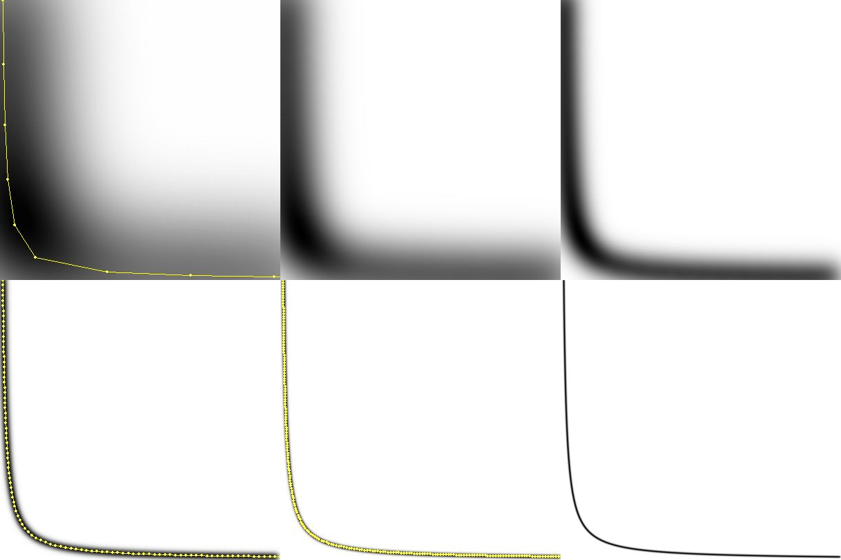
Ideal curves are essentially invisible. However, a quite convenient fuzzyfication ($\overline{\delta}$) of the delta function is the Gauss function: $$ \delta(x) = \lim_{\sigma\rightarrow 0} \norm e^{-\half x^2/\sigma^2} \hieruit \overline{\delta}_\sigma(x) = \norm e^{-\half x^2/\sigma^2} $$ Therefore any discretized curve, at $N$ sampling points $s = s_k$ , can be made approximately continuous again, as follows (apart from a norming factor, which can always be determined afterwards). $$ C(x,y) = \sum_{k=0}^{k=N} e^{-\half([x-f(s_k)]^2+[y-g(s_k)]^2)/\sigma^2} $$ In order for the theory in the preceding subsections to be applicable, it's essential that the points $s_k$ along the curve are more or less equidistant. And if such is not the case, define only one $\sigma$ , which is based then upon the largest arc increment. It's left as an exercise for the reader to guess what the reason is behind these rules. Back to business now. The taste of the pudding is in the eating. You're invited to take a look at the sampled and continuized hyperbola:

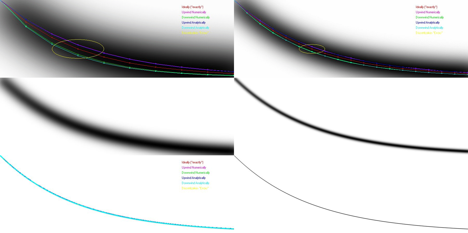
And the sampled and continuized decay function:

There's another story behind the sampled decay function, namely the Numerical Ensemble of Exponential Decays.
A few remarks are in order. The above technique has been developed for curves in the plane. Meaning, physically, that the functions $f$ and $g$ in $(x,y) = [f(s),g(s)]$ have dimension of length. The spread $\sigma$ has a dimension of length as well. Hence the exponent of a Gaussian, as a whole, is dimensionless. With functions instead of curves, other physical dimensions than length may be easily involved. In such cases, proper scaling of the $x$ and $y$ coordinates is essential. One can hardly expect consistent results if f(s) = apples and g(s) = pears. Proper scaling is accomplished most easily and naturally by the use of dimensionless quantities. With exponential decay, for example, the $x$ coordinate is time and the $y$ coordinate is mass; dimensionless quantities emerge if we divide time by the decay time and if we consider a mass of $1$ kilogram.
With Exponential Decay, we had no other choice than leaving the uniform abscissa increments intact, though it leads to arc length increments differing at most by a factor $\sqrt{2}$ (we choose the largest one). With the hyperbola, we have employed a predictorfor abscissa increments, given that the arc length increments $ds$ are constant. Because it is well known that each differentiable function, within a small enough neighborhood, is a straight line segment. Thus our predictor is: $dx = ds / \sqrt{1 + (y')^2} = ds / \sqrt{1 + (1/x^2)^2}$ .