Before trying to be rigorous, it is wise to have some heuristic understanding of the problem:
what is the physical meaning of the Laplace operator?
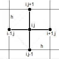
A not too complicated road towards insight is to consider the well known Finite Difference
stencil at a uniform rectangular grid with spacing $h$.
$$
\frac{\partial^2 \phi}{\partial x^2} = \frac{(\phi_{i+1,j}-\phi_{i,j})/h-(\phi_{i,j}-\phi_{i-1,j})/h}{h} \\
\frac{\partial^2 \phi}{\partial y^2} = \frac{(\phi_{i,j+1}-\phi_{i,j})/h-(\phi_{i,j}-\phi_{i,j-1})/h}{h} \\
\frac{\partial^2 \phi}{\partial x^2} + \frac{\partial^2 \phi}{\partial y^2} = 0 \quad \Longrightarrow \\
\left(\phi_{i-1,j}-2\phi_{i,j}+\phi_{i+1,j}\right)+\left(\phi_{i,j-1}-2\phi_{i,j}+\phi_{i,j+1}\right) = 0
\\ \Longrightarrow \quad \phi_{i,j} = \frac{1}{4}\left(\phi_{i-1,j}+\phi_{i+1,j}+\phi_{i,j-1}+\phi_{i,j+1}\right)
$$
It is observed that any value of $\phi$ in the Laplace domain is the mean of its surrounding values.
Quite in general: the Laplace operator $\nabla^2$ is a mean value generator. This becomes even more obvious
if the function $\phi(x,y)$ is identified with a temperature distribution in a heat conducting medium.
The walls at $x=0$ and $x=a$ are insulated, there is a temperature distribution $\phi(x,0)=f(x)$ at the lower boundary
and - from a practical point of view - there is no upper boundary. So what else can happen to the temperature distribution
than flattening out to a mean value in the upper region?
Dejà vu: define the mean value $N$ of the function $f$, a modified function $f^*$
and re-define the OP's second boundary condition:
$$
N(a) = \frac{1}{a} \int_0^a f(x)\,dx \quad ; \quad f^*(x)=f(x)-N(a) \quad ; \quad \phi(x,0) = f^*(x)
$$
Now $f^*(x)$ trivially has mean value zero. And the OP's last boundary condition shall be fulfilled automatically:
$$
\lim_{y\rightarrow\infty}\phi(x,y)=0
$$
Alternatively, one may leave the OP's boundary conditions intact, except for the last one:
$$
\partial_x\phi(0,y)=\partial_x\phi(a,y)=0 \\
\phi(x,0)=f(x) \\
\lim_{y\rightarrow\infty}\phi(x,y)=\frac{1}{a} \int_0^a f(x)\,dx
$$
Function behaviour approaches a constant for $y\to\infty$. Therefore it does no harm to assume a von Neumann BC there:
$\,\lim_{y\rightarrow\infty} \partial_y\phi(x,y)=0\,$.
EDIT.
A numerical solution of the Laplace equation (in rectangular geometry) can be obtained with an equivalent resistor network. Key internet references are found here:
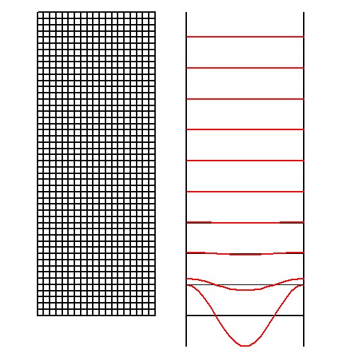
In our case, the domain of interest has been subdivided in little squares:
The predicted "smear out to zero" is clearly visible. And it is pretty fast, suggesting an exponential decay.
Indeed, it is easily verified that the following function obeys the Laplace equation
and it fulfills all boundary conditions as required by the OP:
$$
\phi(x,y)=e^{-2\pi/a.y}\cos\left(\frac{2\pi}{a}x\right)
$$
With exponential decay, little else than a cosine is possible because, together with Boundary Value restrictions:
$$
\phi(x,y) = e^{-ky}f(x) \quad \Longrightarrow \quad \nabla^2 \phi = e^{-ky}\left[\frac{d^2f}{dx^2}+k^2f(x)\right] = 0
$$
Actually, the above analytical solution as a whole can be found with a well known technique: separation of variables.
$$
\phi(x,y)=f(x)g(y) \\
\nabla^2 \phi = \frac{d^2f}{dx^2}g(y)+f(x)\frac{d^2g}{dy^2}=0 \\
\frac{d^2f/dx^2}{f(x)}=-\frac{d^2g/dy^2}{g(y)}=\mbox{constant}=k^2 \\
\frac{d^2f}{dx^2}+k^2f(x)=0 \quad ; \quad \frac{d^2g}{dy^2}-k^2g(y)=0
$$
Solve the ODE's and take care of the BV's.
Our numerical analysis is at the same time a Finite Element Method that comes with a variational principle.
The variational principle for the OP's Laplace equation tries to minimize the following integral over the domain of interest:
$$
\iint \left[\left(\frac{\partial\psi}{\partial x}\right)^2 + \left(\frac{\partial\psi}{\partial y}\right)^2\,\right]dx.dy
$$
An additional feature is that there is a remaining boundary integral, which is zero for so-called natural
boundary conditions. In our case:
$$
\partial_x\phi(0,y)=\partial_x\phi(a,y)=0 \\ \lim_{y\rightarrow\infty} \partial_y\phi(x,y) = 0
$$
Von Neumann boundary conditions zero are fulfilled automatically if, with our numerical method, nothing else is specified.
If we calculate the variational integral for the exact solution as presented, then something very finite indeed comes out
(please check):
$$
\iint \left[\left(\frac{\partial\psi}{\partial x}\right)^2 + \left(\frac{\partial\psi}{\partial y}\right)^2\right]\,dx.dy = \Large \pi
% \\ \iint \left[\left(e^{-2\pi/a.y}.2\pi/a.-\sin(2\pi/a.x)\right)^2 + \left(-2\pi/a.e^{-2\pi/a.y}\cos(2\pi/a.x)\right)^2\right]\,dx.dy =
% \\ \left(\frac{2\pi}{a}\right)^2.\int_0^a\,dx.\int_0^\infty e^{-4\pi/a.y}\,dy = \left(\frac{2\pi}{a}\right)^2.a.\frac{a}{4\pi} = \pi
$$
So perhaps another good requirement may be that the variational integral must be finite.
These are some keyframes. Let other people to do the inbetweening where needed.