CGM = Continuous Geometric Mean. Heuristics and mathematics are described in:
A shortcut to the question as presented here is:
$$
\operatorname{CGM}(\vec{r}) = \exp\left(-\!\!\!\!\!\!\int_0^1 \ln(\left|\vec{p}(t)-\vec{r}\right|^2)\,dt\right)
$$
where $\,\vec{p}(t)\,$ is a circle in the plane and $\,\vec{r} = (x,y)\,$ is another point in the plane.
A similar exercise for the circle as previously for a straight line segment leads to the following expression:
$$
\operatorname{CGM}(\xi,\eta)=
\exp\left( \frac{1}{2\pi}-\!\!\!\!\!\!\int_0^{2\pi}\ln\left|[\cos(t)-\xi]^2+[\sin(t)-\eta]^2\right|\,dt\right)
$$
where dimensionless $\xi=x/R$ , $\eta=y/R$ ; $(x,y)=$ coordinates in the plane, $R=$ radius of circle.
When this expression is fed into MAPLE (version 8),
then surprisingly we get outcome one, independent of any $(x,y,R)$ values:
> exp(int(ln((cos(t)-xi)^2+(sin(t)-eta)^2),t=0..2*Pi,'continuous')/(2*Pi));

                                  1
On the other hand trying to proceed by substituting polar coordinates:
$$
x = r\cos(\phi) \quad ; \quad y = r\sin(\phi) \\
\exp\left(\frac{1}{2\pi}-\!\!\!\!\!\!\int_0^{2\pi} \ln\left|\left[\cos(t)-\frac{r}{R}\cos(\phi)\right]^2
+\left[\sin(t)-\frac{r}{R}\sin(\phi)\right]^2\right|\,dt\right)
\quad \Longrightarrow \\ \operatorname{CGM}(\rho) =
\exp\left(\frac{1}{2\pi}-\!\!\!\!\!\!\int_0^{2\pi} \ln\left|\rho^2+1-2\rho.\cos(t-\phi)\right|\,dt\right)
\quad \mbox{with} \quad \rho=r/R
$$
Because of circle symmetry we can choose $\,\phi=0\,$ without loss of generality.
Care should be taken if a zero is present in the argument of the logarithm, resulting in a singularity at that place:
$$
\rho^2+1-2\rho.\cos(t)=0 \quad \Longrightarrow \quad \rho = \cos(t)\pm\sqrt{\cos^2(t)-1}
\\ \Longrightarrow \quad t = 0 \quad \mbox{and} \quad \rho = 1
$$
There are two approaches to this special case.
The easiest one is to ignore the Cauchy principal value and remember that
the special case represents the value zero, according to the heuristics in the referenced
Q&A.
The second approach is to accept the Cauchy principal value as being essential.
With our numerical method, being the trapezium rule, integration at the interval $[0,\Delta t]$ is then calculated by:
$$
\frac{f_1+f_2}{2}\Delta t \quad \mbox{with} \quad f_2 = \ln|2-2\cos(\Delta t)| \approx \ln|2-2(1-\Delta t^2/2)| = 2\ln|\Delta t|
$$
On the other hand the integral at that place can be calculated more (or less) exactly:
$$
\frac{f_1+f_2}{2}\Delta t \approx \int_0^{\Delta t}\ln|2-2\cos(t)|\,dt \approx
\int_0^{\Delta t}2\ln|t|\,dt = 2(\Delta t\,\ln|\Delta t| - \Delta t) \\
\frac{f_1+2\ln|\Delta t|}{2}\Delta t \approx 2(\ln|\Delta t|-1)\Delta t \quad \Longrightarrow \quad f_1 \approx 2\ln|\Delta t|-4
$$
Having programmed all this (in Delphi Pascal) we get the following output.
Mind the two bold printed values at $I(1.0)$ : the first one without and the second one with the Cauchy principal value.
          NUMERICALLY               CONJECTURED
I(0.0) =  1.00000000000000E+0000 =  1.00000000000000E+0000
I(0.1) =  1.00000000000000E+0000 =  1.00000000000000E+0000
I(0.2) =  1.00000000000000E+0000 =  1.00000000000000E+0000
I(0.3) =  1.00000000000000E+0000 =  1.00000000000000E+0000
I(0.4) =  1.00000000000000E+0000 =  1.00000000000000E+0000
I(0.5) =  1.00000000000000E+0000 =  1.00000000000000E+0000
I(0.6) =  9.99999999999999E-0001 =  1.00000000000000E+0000
I(0.7) =  1.00000000000000E+0000 =  1.00000000000000E+0000
I(0.8) =  1.00000000000000E+0000 =  1.00000000000000E+0000
I(0.9) =  1.00000000000000E+0000 =  1.00000000000000E+0000
I(1.0) =  0.00000000000000E+0000 =  0.00000000000000E+0000
I(1.0) =  9.99967575938953E-0001 =  1.00000000000000E+0000
I(1.1) =  1.21000000000000E+0000 =  1.21000000000000E+0000
I(1.2) =  1.44000000000000E+0000 =  1.44000000000000E+0000
I(1.3) =  1.69000000000000E+0000 =  1.69000000000000E+0000
I(1.4) =  1.96000000000000E+0000 =  1.96000000000000E+0000
I(1.5) =  2.24999999999999E+0000 =  2.25000000000000E+0000
I(1.6) =  2.55999999999999E+0000 =  2.56000000000000E+0000
I(1.7) =  2.89000000000002E+0000 =  2.89000000000000E+0000
I(1.8) =  3.24000000000002E+0000 =  3.24000000000000E+0000
I(1.9) =  3.61000000000001E+0000 =  3.61000000000000E+0000
I(2.0) =  4.00000000000000E+0000 =  4.00000000000000E+0000
I(2.1) =  4.41000000000001E+0000 =  4.41000000000000E+0000
I(2.2) =  4.84000000000001E+0000 =  4.84000000000000E+0000
I(2.3) =  5.29000000000000E+0000 =  5.29000000000000E+0000
I(2.4) =  5.75999999999996E+0000 =  5.76000000000000E+0000
I(2.5) =  6.24999999999998E+0000 =  6.25000000000000E+0000
I(2.6) =  6.75999999999999E+0000 =  6.76000000000001E+0000
I(2.7) =  7.29000000000010E+0000 =  7.29000000000001E+0000
I(2.8) =  7.84000000000007E+0000 =  7.84000000000001E+0000
I(2.9) =  8.41000000000004E+0000 =  8.41000000000001E+0000
I(3.0) =  9.00000000000000E+0000 =  9.00000000000001E+0000
The numerical experiments give rise to the following conjecture (contradictory on purpose):
$$
\operatorname{CGM}(\rho) = \begin{cases} 1 & \mbox{for} \quad \rho \le 1 \\ 0 & \mbox{for} \quad \rho = 1 \\
\rho^2 & \mbox{for} \quad \rho \ge 1 \end{cases}
$$
Is there someone who can prove this conjecture analytically?
I have seen something with complex analysis in
sci.math a long time ago (2008) but didn't quite understand the argument.
CGM for a Sphere
In view of further development of the theory, it seems to be advantageous to define the Continuous Geometric Mean slightly different, namely as:
$$
\operatorname{CGM}(\vec{r}) = \exp\left(- -\!\!\!\!\!\!\int_0^1 \ln(\left|\vec{p}(t)-\vec{r}\right|^2)\,dt\right)
$$
For our unit circle (with Cauchy principal value) then we have instead:
$$
\operatorname{CGM}(\rho) = \begin{cases} 1 & \mbox{for} \quad \rho \le 1 \\ 1/\rho^2 & \mbox{for} \quad \rho \ge 1 \end{cases}
$$
We seek to generalize the Continuous Geometric Mean for a circle to the same for the surface of a unit sphere:
$$
\operatorname{CGM}(\vec{r}) = \exp\left(-\iint \ln(\left|\vec{p}-\vec{r}\right|^2)\,dA/(4\pi)\right)
$$
Expressed in spherical coordinates and specializing (without loss of generality) for $\,\vec{r} = (0,0,\rho)\,$:
$$
\vec{p}-\vec{r} = \begin{bmatrix} \sin(\theta)\cos(\phi) \\ \sin(\theta)\sin(\phi) \\ \cos(\theta)-\rho \end{bmatrix}
\quad ; \quad dA = \sin(\theta)\,d\theta\,d\phi \\
\left|\vec{p}-\vec{r}\right|^2 = \sin^2(\theta)+\left[\,\cos(\theta)-\rho\,\right]^2 = 1-2\rho\cos(\theta)+\rho^2 \\
\iint \ln(\left|\vec{p}-\vec{r}\right|^2)\,dA / (4\pi)=
\frac{2\pi}{4\pi} -\!\!\!\!\!\!\!\int_0^\pi \ln\left|\rho^2+1-2\rho\,\cos(\theta)\right|\,\sin(\theta)\,d\theta
\\ \Longrightarrow \quad
\operatorname{CGM}(\rho) = \exp\left(-\frac{1}{2} -\!\!\!\!\!\!\!\int_0^{\pi} \ln\left|\rho^2+1-2\rho\,\cos(\theta)\right|\,\sin(\theta)\,d\theta\right)
$$
Surprisingly enough, integration is much easier in 3-D, when compared with the 2-D case. Substitution of $\,t = \cos(\theta)\,$ gives a short route to the solution:
$$
-\!\!\!\!\!\!\int_0^{\pi} \ln\left|\rho^2+1-2\rho\,\cos(\theta)\right|\,\sin(\theta)\,d\theta =
-\!\!\!\!\!\!\int_{-1}^{+1}\ln\left|\rho^2+1-2\rho\,t\right|\,dt = \\
\frac{1}{2\rho}\left[\;u\ln|u|-u\;\right]_{u=1+\rho^2-2\rho}^{u=1+\rho^2+2\rho} \quad \Longrightarrow \\
\operatorname{CGM}(\rho) = \exp\left(-\left[(1+\rho)^2\ln\left|(1+\rho)^2\right|-(1-\rho)^2\ln\left|(1-\rho)^2\right|-4\rho\right]/(4\rho)\right)
$$
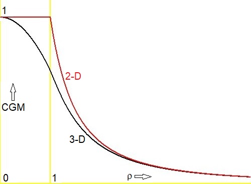
If we make a graph of the two functions - red for 2-D, black for 3-D - then there is another surprise: the graphs coincide for large values of the normed radius $\rho$.
Confirmation is found with MAPLE, series expansion for $q=1/\rho\to 0$:
> f(q) := exp(-((1+1/q)^2*ln((1+1/q)^2)-(1-1/q)^2*ln((1-1/q)^2)-4/q)/(4/q));
> series(f(q),q=0);
Output:
$$
({q}^{2}-{\frac {1}{3}}{q}^{4}+O \left( {q}^{6} \right) )
$$
Here comes a replay of Richard Feynman's Integral Trick, adapted ( if not improved ) for our purpose. Define:
$$
I(a)=\int_{0}^{2\pi}\ln\left(1-2a\cos x+a^2\right)\ \mathrm{d}x \quad , \quad a \ge 0
$$
Then
\begin{align}
I'(a)&=\int_{0}^{2\pi}\frac{2a-2\cos x}{1-2a\cos x+a^2} \ \mathrm{d}x \\
& = \frac{1}{a}\int_{0}^{2\pi}\frac{2a^2-2a\cos x}{1-2a\cos x+a^2} \ \mathrm{d}x \\
& = \frac{1}{a}\int_{0}^{2\pi}\frac{1-1+a^2+a^2-2a\cos x}{1-2a\cos x+a^2} \ \mathrm{d}x \\
& = {2\pi \over a} + \frac{1}{a}\int_{-\pi}^{+\pi}\frac{a^2-1}{1-2a\cos x+a^2} \ \mathrm{d}x
\end{align}
and making the Weierstrass substitution:
$$t = \tan(x/2)$$
$$t^2\cos^2(x/2)=\sin^2(x/2)=1-\cos^2(x/2)$$
$$\cos^2(x/2)=\frac{1}{1+t^2}$$
$$\cos(x)=2\cos^2(x/2)-1$$
$$\cos x = \frac{1 - t^2}{1 + t^2},$$
$$x=2\,\arctan(t)$$
$$\mathrm{d}x = \frac{2 \,\mathrm{d}t}{1 + t^2}.$$
\begin{align}
I'(a)&={2\pi \over a} + \frac{2}{a}\int_{-\infty}^{+\infty}\frac{a^2-1}{(1+a^2)(1+t^2)-2a(1-t^2)}\ \mathrm{d}t \\
&={2\pi \over a} + \frac{2}{a}\int_{-\infty}^{+\infty}\frac{a^2-1}{(1-a)^2 + (1+a)^2t^2} \ \mathrm{d}t \\
&={2\pi \over a} + \frac{2}{a}\frac{a^2-1}{(1-a)^2}2\int_{0}^{\infty}\frac{dt}{1 + \left|(1+a)/(1-a).t\right|^2}
\end{align}
Two cases are to be distinguished:
$$
\begin{cases} a \lt 1 & : & u = \left|(1+a)/(1-a).t\right| = (1+a)/(1-a).t \\
a \gt 1 & : & u = \left|(1+a)/(1-a).t\right| = (1+a)/(a-1).t \end{cases}
$$
For $\,a\lt\ 1\,$:
$$
I'(a)={2\pi \over a} + \frac{4}{a}\frac{(a+1)(a-1)(1-a)}{(1-a)^2(1+a)}\int_{0}^{\infty}\frac{du}{1+u^2}\\
={2\pi \over a}-\frac{4}{a}\left[\,\arctan(u)\,\right]_{u=0}^{u=\infty}={2\pi \over a}-\frac{4}{a}\frac{1}{2}\pi=0 $$
$$ \Longrightarrow \quad I(a) = C$$
For $\,a\gt\ 1\,$:
$$
I'(a)={2\pi \over a} + \frac{4}{a}\frac{(a+1)(a-1)(a-1)}{(1-a)^2(1+a)}\frac{1}{2}\pi=\frac{4\pi}{a}
$$ $$ \Longrightarrow \quad I(a) = 4\pi\ln(a) + C
$$
where $\,C\,$ is an integration constant, to be determined for $\,a=0\,$:
$$
C = I(a=0)=\int_{0}^{2\pi}\ln\left(1-2a\cos x+a^2\right)\ \mathrm{d}x \\ = \int_{0}^{2\pi}\ln\left(1\right)\ \mathrm{d}x = 0
$$
End result:
$$
I(a)=\int_{0}^{2\pi}\ln\left(1-2a\cos x+a^2\right)\ \mathrm{d}x =
\begin{cases}0 & \mbox{for } \; a \lt 1 \\ 2\pi\,\ln\left(a^2\right) & \mbox{for } \; a \gt 1 \end{cases}
$$
The special case $\,a=1\,$.
$$
I(a=1)=\int_{0}^{2\pi}\ln\left(1-2a\cos x+a^2\right)\ \mathrm{d}x \\ =
\int_{0}^{2\pi}\ln\left(2-2\cos x \right)\ \mathrm{d}x\\
=\int_{0}^{2\pi}\ln\left(4\sin^2\frac12 x\right)\ \mathrm{d}x =
2\int_{0}^{\pi}\ln\left(4\sin^2 t\right)\ \mathrm{d}t\\
=2(\ln 4)\pi+\color{red}{4\int_{0}^{\pi}\ln\left(\sin t\right)\ \mathrm{d}t}
=\color{red}{4\pi\ln 2} +8\int_{0}^{\pi/2}\ln\left(\sin t\right)\ \mathrm{d}t\\
=4\pi\ln 2 +8\left[\int_{0}^{\pi/2}\ln\left(\sin t\right)\ \mathrm{d}t + \int_{0}^{\pi/2}\ln\left(\cos t\right)\ \mathrm{d}t\right]/2\\
=4\pi\ln 2 +4\int_{0}^{\pi/2}\ln\left(\sin t\cos t\right)\ \mathrm{d}t\\
=4\pi\ln 2 +4\int_{0}^{\pi/2}\ln\left(\frac12 \sin 2t\right)\ \mathrm{d}t\\
=4\pi\ln 2 +4\ln\left(\frac12\right)\frac{\pi}{2}+4\frac12\int_{0}^{\pi}\ln\left(\sin x\right)\ \mathrm{d}x\\
=2\pi\ln 2 +2\int_{0}^{\pi}\ln\left(\sin x\right)\ \mathrm{d}x
=\color{red}{4\pi\ln 2 +4\int_{0}^{\pi}\ln\left(\sin t\right)\ \mathrm{d}t}\\
\Longrightarrow \quad \int_{0}^{\pi}\ln\left(\sin t\right)\ \mathrm{d}t = -\pi\ln 2 \\
\Longrightarrow \quad I(a=1)= 4\pi\ln 2 + 4\int_{0}^{\pi}\ln\left(\sin t\right)\ \mathrm{d}t = 0
$$