Double refinement of Nesbitt's inequality

Define a (real valued) function $F(a,b,c)$ and re-define the inequality as follows: $$ F(a,b,c) = \frac{a}{\sqrt[3]{4(b^3+c^3)}}+\frac{b}{a+c}+\frac{c}{a+b} - \sqrt{\frac94+\frac{(a-b)^2}{ab+bc+ca}} \geq 0 $$ Define new variables $x = a/c$ and $y = b/c$. Due to the restrictions for $a,b,c$, and scaling properties of $F$, the problem can be rewritten as a two-dimensional one: $$ f(x,y) = \frac{x}{\left[(4(y^3+1)\right]^{1/3}}+\frac{y}{x+1}+\frac{1}{x+y}-\sqrt{\frac{9}{4}+\frac{(x-y)^2}{xy+x+y}} \geq 0 $$ With $1 \leq y \leq 2$ and $x \gt 0$.
So the problem boils down to an investigation of function behaviour in 2-D.
To get a first impression, we start with a pictorial exercise: contouring of the function. After some attempts, it seems that the following window may be interesting:

  xmin := 0; xmax := 2;
  ymin := 1; ymax := 2;

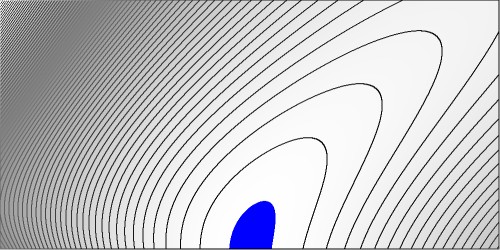
Maximum and minimum vales of $f(x,y)$ are determined first and the place of the minimum is estimated numerically:

 1.39061000309967E-0007 < f < 4.38447187191170E-0001
f( 1.00100100100100E+0000, 1.00200803212851E+0000) =  1.39061000309967E-0007

There are $75$ (vertically) equidistant isolines between the minimum and the maximum. The picture is colored blue for funcion values $f(x,y) < 0.001$. It is suggested - not formally proved - that maybe a global minimum equal to zero is found for $x$ and $y$ equal to one: $f(1,1)=0$. Let's check this. A computer algerba system (MAPLE) has been employed when calculations became tedious (and essentially uninteresting as well):

> f(x,y) := x/((4*(y^3+1))^(1/3))+y/(x+1)+1/(x+y)-sqrt(9/4+(x-y)^2/(x*y+x+y));
> simplify(subs(x=1,y=1,f(x,y)));
                                       0

Meaning that the exact value of $f(1,1)$ is zero, as expected.
Next calculate the partial derivatives $\;\large\frac{\partial f}{\partial x}\small (1,1)\;$ and $\;\large\frac{\partial f}{\partial y}\small (1,1)\;$. Verify that they are zero:

> simplify(subs(x=1,y=1,diff(f(x,y),x)));
                                               0
> simplify(subs(x=1,y=1,diff(f(x,y),x)));
                                               0

Calculate the second order partial derivatives $\;\large\frac{\partial^2 f}{\partial x^2}\small(1,1)\;$ , $\;\large\frac{\partial^2 f}{\partial y^2}\small(1,1)\;$ , $\;\large\frac{\partial^2 f}{\partial x \partial y}\small(1,1)\;$:

> simplify(subs(x=1,y=1,diff(diff(f(x,y),x),x)));
                                                      5/18
> simplify(subs(x=1,y=1,diff(diff(f(x,y),y),y)));
                                                      1/36
> simplify(subs(x=1,y=1,diff(diff(f(x,y),x),y)));
> simplify(subs(x=1,y=1,diff(diff(f(x,y),y),x)));
                                                    - 1/36

So the Hessian matrix of our function at $(1,1)$ is: $$ \begin{bmatrix} +5/18 & -1/36 \\ -1/36 & +1/36 \end{bmatrix} $$ The Hessian is positive definite here, because of its eigenvalues $\lambda_1,\lambda_2$: $$ \left.\begin{matrix} \mbox{Trace} = \lambda_1 + \lambda_2 &=& 5/18 + 1/36 = 11/36 > 0 \\ \mbox{Determinant} = \lambda_1 . \lambda_2 &=& 5/18.1/36 - (1/36)^2 = 9/36^2 > 0 \end{matrix}\right\} \Longrightarrow \lambda_1 > 0 \; , \; \lambda_2 > 0 $$ This ensures that we have found indeed a (local) minimum.

Inspection at the left side of the picture - i.e. for $\;x \downarrow 0\;$ - shows that there is no reason to assume that function values $f(x,y)$ become somehow close to zero there. But it's not forbidden to investigate e.g. 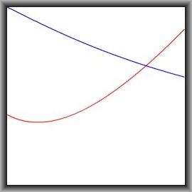the borderline case: $$ \lim_{x\to 0} \left\{ \frac{x}{\left[(4(y^3+1)\right]^{1/3}}+\frac{y}{x+1}+\frac{1}{x+y}-\sqrt{\frac{9}{4}+\frac{(x-y)^2}{xy+x+y}} \right\} \\ = y + \frac{1}{y} - \sqrt{\frac{9}{4} + y} $$ In view of this, define the function $\color{red}{f(x) = x + 1/x - \sqrt{9/4 + x}}$.
There is no such borderline case at the right side of the picture, because the $x$-coordinate has no upper bound. So there might be uncertainty for larger values of $x$, formally $\; x \to \infty\;$. To gain more insight, we calculate the following limit, because it is suspected that the first term is dominant: $$ \lim_{x\to\infty} \left\{ \frac{x}{\left[(4(y^3+1)\right]^{1/3}}+\frac{y}{x+1}+\frac{1}{x+y}-\sqrt{\frac{9}{4}+\frac{(x-y)^2}{xy+x+y}} \right\}\large / x \\ = \lim_{x\to\infty} \left\{ \frac{1}{\left[(4(y^3+1)\right]^{1/3}}+\frac{y}{x(x+1)}+\frac{1}{x(x+y)}-\sqrt{\frac{9}{4x^2}+\frac{(1-y/x)^2}{xy+x+y}} \right\} \\ = \frac{1}{\left[(4(y^3+1)\right]^{1/3}} $$ In view of this, define the function $\color{blue}{g(x) = 1/\left[(4(x^3+1)\right]^{1/3}}$.
Both functions are displayed in the picture below, for $0 < x < 2$ and $0 < y < 5$, to ensure that both are positive valued (which by the way is trivial for the blue one). It is noticed that the red function has a minimum above zero. Of course $\color{red}{f(x)}$ and $\color{blue}{g(x)}$ can be investigated analytically as well, but without a computer algebra system it quickly becomes complicated and hence error prone. What's worse: there is hardly any additional value. That's why I prefer the graphics:

For $x\to\infty$ it is concluded that there are no values near zero in that far away region. But where does the far away region start? To settle this issue, consider the expression: $$ \delta(x,y) = 1 - \frac{\left[(4(y^3+1)\right]^{1/3}}{x} \times \\ \left\{ \frac{x}{\left[(4(y^3+1)\right]^{1/3}}+\frac{y}{x+1}+\frac{1}{x+y}-\sqrt{\frac{9}{4}+\frac{(x-y)^2}{xy+x+y}} \right\} $$ Or, alternatively (approximately the same for large $x$-values) : $$ \delta(x,y) = \ln\left(\frac{x}{\left[(4(y^3+1)\right]^{1/3}}\right) - \\ \ln\left(\frac{x}{\left[(4(y^3+1)\right]^{1/3}}+\frac{y}{x+1}+\frac{1}{x+y}-\sqrt{\frac{9}{4}+\frac{(x-y)^2}{xy+x+y}}\right) $$ with the interpretation attached that $\delta$ is a relative error of the limiting value $x/\left[(4(y^3+1)\right]^{1/3}$. Then perform numerical experiments for $1 \leq y \leq 2$ (as usual) and for $x = 10$, giving: $\delta \lt 90\,\%\;$. Ongoing from there, $\delta$ is continuously decreasing with increasing $x$, as expected. There is enough margin in the blue $\color{blue}{g(x)}$ to ensure that any $\delta(x,y)$ for $x \gt 10$ do not make it close to zero. So we only have to investigate function behaviour for say $0 \lt x \leq 10$, a limited range of $(x,y)$ values.

Having done all this, we must conclude that the Double refinement of Nesbitt's inequality, as proposed by the OP, is valid.