2-D Resistor Model
$
\def \half {\frac{1}{2}}
\newcommand{\dq}[2]{\displaystyle \frac{\partial #1}{\partial #2}}
\def \J {\Delta}
$
Consider the two-dimensional equation (or term), which describes, for example,
conduction of heat in a metal plate:
$$
\dq{}{x} \left[ - \lambda \dq{T}{x} \right]
+ \dq{}{y} \left[ - \lambda \dq{T}{y} \right] = 0
$$
Here $(x,y) = $ planar Cartesian coordinates, $\lambda = $ conductivity, $T = $
temperature. In general, the conductivity is also a function $\lambda(x,y)$ of
the coordinates $x$ and $y$ . The equation is of the form:
$$
\dq{Q_x}{x} + \dq{Q_y}{y} = 0
$$
Where:
$$
Q_x = - \lambda \dq{T}{x} \quad ; \quad Q_y = - \lambda \dq{T}{y}
$$
This equation has already been treated in the section "Conservation of Heat".
Application of the Galerkin method there resulted in:
$$
- \half \left[ \begin{array}{ccc} f_1 & f_2 & f_3 \end{array} \right]
\left[ \begin{array}{cc} y_2 - y_3 & x_3 - x_2 \\
y_3 - y_1 & x_1 - x_3 \\
y_1 - y_2 & x_2 - x_1 \end{array} \right]
\left[ \begin{array}{c} Q_x \\ Q_y \end{array} \right]
$$
Discretization of $Q_x$ and $Q_y$, with help of the Differentiation Matrix of
a triangle, gives, in addition:
$$
\left[ \begin{array}{c} Q_x \\ Q_y \end{array} \right] = - \lambda
\left[ \begin{array}{ccc} y_2 - y_3 & y_3 - y_1 & y_1 - y_2 \\
x_3 - x_2 & x_1 - x_3 & x_2 - x_1 \end{array}
\right] / \J
\left[ \begin{array}{c} T_1 \\ T_2 \\ T_3 \end{array} \right]
$$
In order to save space, the following abbreviations will be used:
$x_{ij} = x_j - x_i$ , $y_{ij} = y_j - y_i$ . Then the Analytical expression:
$$
\dq{}{x} \left[ - \lambda \dq{T}{x} \right]
+ \dq{}{y} \left[ - \lambda \dq{T}{y} \right]
$$
corresponds with the Numerical expression:
$$
- \half \left[ \begin{array}{ccc} f_1 & f_2 & f_3 \end{array} \right]
\left[ \begin{array}{cc} y_{32} & x_{23} \\
y_{13} & x_{31} \\
y_{21} & x_{12} \end{array} \right]
. \: - \lambda \: .
\left[ \begin{array}{ccc} y_{32} & y_{13} & y_{21} \\
x_{23} & x_{31} & x_{12} \end{array}
\right] / \J
\left[ \begin{array}{c} T_1 \\ T_2 \\ T_3 \end{array} \right]
$$ $$
= +
\left[ \begin{array}{ccc} f_1 & f_2 & f_3 \end{array} \right] \half
\left[ \begin{array}{ccc} E_{11} & E_{12} & E_{13} \\
E_{21} & E_{22} & E_{23} \\
E_{31} & E_{32} & E_{33} \end{array} \right]
. \lambda / \J
\left[ \begin{array}{c} T_1 \\ T_2 \\ T_3 \end{array} \right]
$$
The finite element matrix $\left[ E_{ij} \right]$ is thus defined,
in our case, by:
$$
\half
\left[ \begin{array}{ccc} y_{23}.y_{23} + x_{23}.x_{23} &
y_{23}.y_{31} + x_{23}.x_{31} &
y_{23}.y_{12} + x_{23}.x_{12} \\
&
y_{31}.y_{31} + x_{31}.x_{31} &
y_{31}.y_{12} + x_{31}.x_{12} \\
\mbox{symmetrical} &
&
y_{12}.y_{12} + x_{12}.x_{12} \end{array} \right]
. \lambda / \J
$$
A possible interpretation, for an arbitrary matrix coefficient, may be obtained
as follows:
$$
E_{23} = E_{32} = \half \left( y_{31}.y_{12} + x_{31}.x_{12} \right)
. \lambda / \J
$$ $$
= \half \left[ (x_2 - x_1).(x_1 - x_3) + (y_2 - y_1).(y_1 - y_3) \right]
. \lambda / \J
$$ $$
= - \half ( \vec{r}_{12} \cdot \vec{r}_{13} )
. \lambda / \J
$$
And for main diagonal elements:
$$
E_{33} = \half \left( y_{12}.y_{12} + x_{12}.x_{12} \right)
. \lambda / \J
$$ $$
= \half \left[ (x_2 - x_1).(x_2 - x_1) + (y_2 - y_1).(y_2 - y_1) \right]
. \lambda / \J
$$ $$
= + \half ( \vec{r}_{12} \cdot \vec{r}_{12} )
. \lambda / \J
$$
Since any vertex of the triangle is equally important, remaining coefficients
may be found by cyclic permutation of the vertex indices, according to
$(1,2,3) \rightarrow (2,3,1) \rightarrow (3,1,2)$ :
\begin{eqnarray*}
E_{31} = E_{13} = - \half ( \vec{r}_{23} \cdot \vec{r}_{21} )
. \lambda / \J \\
E_{12} = E_{21} = - \half ( \vec{r}_{31} \cdot \vec{r}_{32} )
. \lambda / \J \\
E_{11} = + \half ( \vec{r}_{23} \cdot \vec{r}_{23} )
. \lambda / \J \\
E_{22} = + \half ( \vec{r}_{31} \cdot \vec{r}_{31} )
. \lambda / \J
\end{eqnarray*}
With other words: any matrix element is the inner product of vectors
pointing from one vertex to one ($+$) or two ($-$) other vertices.
It is
remarked that, according to one of Patankar's "Four Basic Rules" [SV],
namely "the rule of positive coefficients", off-diagonal terms $E_{ij}$ with
$i \ne j$ must be less than zero. This is only the case for positive
inner products $ ( \vec{r}_{ki} \cdot \vec{r}_{kj} ) $, assuming that the
determinants $ \J $ are positive (: a convention that we have already agreed
upon). This implies that any angle of a Diffusion Triangle must be $ \le 90^o $.
A special case occurs when the angle between the vectors $ \vec{r}_{ki} $ and
$ \vec{r}_{kj} = $ 90 degrees, which means that $E_{ij} = 0$. This is actually
the finite difference case, on a rectangular grid: "no" triangles, but five
point stars "instead".
Almost any Finite Element book starts with the assembly of resistor-like finite
elements, without approximations (if one considers Ohm's law as being "exact").
Contained in [NdV] is a chapter about
"Electrical Networks". The matrix
of an electrical resistor is derived there directly by applying the laws
of Ohm and Kirchhoff, giving:
$$
\left[ \begin{array}{cc} + 1/R & - 1/R \\
- 1/R & + 1/R \end{array} \right]
$$
where $R$ are the resistances. \\
Further define the connectivity (no coordinates!) of the resistor-network, and
apply two voltages. The standard FE assembly procedure can be carried out then.
Let us devise for example a triangle, built up from electrical resistors:
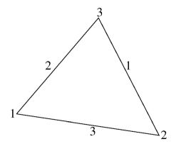
Opposite sides and vertices are numbered alike, which is nothing but a handsome
practice. The accompanying resistor matrices are subsequently added together,
to form the (finite element) resistor matrix of the triangle as a whole:
$$
\left[ \begin{array}{ccc} 0 & 0 & 0 \\
0 & + 1/R_1 & - 1/R_1 \\
0 & - 1/R_1 & + 1/R_1 \end{array} \right] +
\left[ \begin{array}{ccc} + 1/R_2 & 0 & - 1/R_2 \\
0 & 0 & 0 \\
- 1/R_2 & 0 & + 1/R_2 \end{array} \right] +
\left[ \begin{array}{ccc} + 1/R_3 & - 1/R_3 & 0 \\
- 1/R_3 & + 1/R_3 & 0 \\
0 & 0 & 0 \end{array} \right]
$$ $$
= \left[ \begin{array}{ccc} + 1/R_2 + 1/R_3 & - 1/R_3 & - 1/R_2 \\
- 1/R_3 & + 1/R_3 + 1/R_1 & - 1/R_1 \\
- 1/R_2 & - 1/R_1 & + 1/R_1 + 1/R_2
\end{array} \right]
$$
It is trivially seen that:
$$
E_{11} + E_{12} + E_{13} = 0 \quad ; \quad
E_{12} + E_{22} + E_{23} = 0 \quad ; \quad
E_{31} + E_{32} + E_{33} = 0
$$
Compare this result with our previous findings:
$$
\half
\left[ \begin{array}{ccc} y_{32}.y_{32} + x_{32}.x_{32} &
y_{32}.y_{13} + x_{32}.x_{13} &
y_{32}.y_{21} + x_{32}.x_{21} \\
&
y_{13}.y_{13} + x_{13}.x_{13} &
y_{13}.y_{21} + x_{13}.x_{21} \\
\mbox{symmetrical} &
&
y_{21}.y_{21} + x_{21}.x_{21} \end{array} \right]
.\lambda / \J $$
It is questioned if all terms in a matrix row sum up to zero here too.
There are a myriad ways to see that this is indeed the case. According to one
of Patankar's "Basic Rules", the coefficients sum up to zero without question.
One can work out each term algebraically and check out. A more elegant way is
via geometrical interpretation. Draw the perpendicular $\overline{CH}$ from
vertex $C$ onto $\overline{AB}$ :
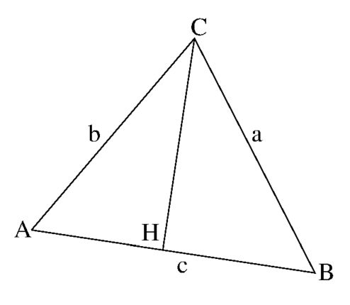
Take the third matrix row as an example:
$$
E_{31} = E_{13} = - \half c.a.cos(B) . \lambda / \J \quad ; \quad
E_{32} = E_{23} = - \half c.b.cos(A) . \lambda / \J
$$ $$
E_{31} + E_{32} = - \half c.(\overline{AH} + \overline{BH} ) . \lambda / \J
= - \half c.c .\lambda / \J = - \, E_{33}
$$
Now identify:
\begin{eqnarray*}
\half (y_{23}.y_{31} + x_{23}.x_{31}) / \J = - 1/R_3
\quad \mbox{or} \quad R_3 = \frac{2 \J / \lambda }{a.b.cos(C)} \\
\half (y_{23}.y_{12} + x_{23}.x_{12}) / \J = - 1/R_2
\quad \mbox{or} \quad R_2 = \frac{2 \J / \lambda }{a.c.cos(B)} \\
\half (y_{31}.y_{12} + x_{31}.x_{12}) / \J = - 1/R_1
\quad \mbox{or} \quad R_1 = \frac{2 \J / \lambda }{b.c.cos(A)} \\
\end{eqnarray*}
Thus we can consider the $3 \times 3$ matrix for diffusion at a triangle as a
superposition of one-dimensional resistor-like elements (an outstanding example
of substructuring, anyway).
When assembling these triangle matrices into the global system, most resistors
have to be replaced by two parallel resistors, one resistor for each side of a
triangle, according to the law: $ 1/R = 1/R_a + 1/R_b $. Exceptions are at the
boundary.
The main diagonal term in a matrix equals the sum of the off-diagonal terms.
This result can be used as follows: account only for the off-diagonal
terms in the first place. At the very end of the F.E. assembly procedure,
sum up each matrix row, in order to obtain the main diagonal elements.