Substitute $ x=x_k $ and $ y=y_k $ with $ k=1,2,3 $:
$$
\left[ \begin{array}{c} T_1 \\ T_2 \\ T_3 \end{array} \right] =
\left[ \begin{array}{ccc} 1 & x_1 & y_1 \\
1 & x_2 & y_2 \\
1 & x_3 & y_3 \end{array} \right]
\left[ \begin{array}{c} C \\ A \\ B \end{array} \right]
$$
The first of these equations can already be used to eliminate the
constant $C$, once and forever:
$$
T_1 = A.x_1 + B.y_1 + C
$$
Resulting in:
$$
T - T_1 = A.(x - x_1) + B.(y - y_1)
$$
Hence the constants $A$ and $B$ are determined by:
$$ \begin{array}{ll}
T_2 - T_1 = A.(x_2 - x_1) + B.(y_2 - y_1) \\
T_3 - T_1 = A.(x_3 - x_1) + B.(y_3 - y_1)
\end{array} $$
Two equations with two unknowns. The solution is found by straightforward
elimination, or by applying Cramer's rule:
$$ \begin{array}{ll}
A = [ (y_3 - y_1).(T_2 - T_1) - (y_2 - y_1).(T_3 - T_1) ] / \Delta \\
B = [ (x_2 - x_1).(T_3 - T_1) - (x_3 - x_1).(T_2 - T_1) ] / \Delta
\end{array} $$
There are several forms of the determinant $\Delta$, which should be memorized when
it is appropriate:
\begin{eqnarray*}
&& \Delta = (x_2 - x_1).(y_3 - y_1) - (x_3 - x_1).(y_2 - y_1) \\
&& \Delta = 2 \times \mbox{ area of triangle } \\
&& \Delta = x_1.y_2 + x_2.y_3 + x_3.y_1 - y_1.x_2 - y_2.x_3 - y_3.x_1 \\
&& \Delta = x_1.(y_2 - y_3) + x_2.(y_3 - y_1) + x_3.(y_1 - y_2) \\
&& \Delta = y_1.(x_3 - x_2) + y_2.(x_1 - x_3) + y_3.(x_2 - x_1) \\
&& \Delta = \left\| \begin{array}{ccc} 1 & x_1 & y_1 \\
1 & x_2 & y_2 \\
1 & x_3 & y_3 \end{array} \right\|
\end{eqnarray*}
Anyway, it is concluded that:
$$
T - T_1 = \xi.(T_2 - T_1) + \eta.(T_3 - T_1)
$$ Where:
$$ \begin{array}{ll}
\xi = [ (y_3 - y_1).(x - x_1) - (x_3 - x_1).(y - y_1) ] / \Delta \\
\eta = [ (x_2 - x_1).(y - y_1) - (y_2 - y_1).(x - x_1) ] / \Delta
\end{array} $$
Or:
$$
\left[ \begin{array}{c} \xi \\ \eta \end{array} \right] =
\left[ \begin{array}{cc} + (y_3 - y_1) & - (x_3 - x_1) \\
- (y_2 - y_1) & + (x_2 - x_1)
\end{array} \right] / \Delta
\left[ \begin{array}{c} x - x_1 \\ y - y_1 \end{array} \right]
$$
The inverse of the following problem is recognized herein:
$$
\left[ \begin{array}{c} x - x_1 \\ y - y_1 \end{array} \right] =
\left[ \begin{array}{cc} (x_2 - x_1) & (x_3 - x_1) \\
(y_2 - y_1) & (y_3 - y_1)
\end{array} \right]
\left[ \begin{array}{c} \xi \\ \eta \end{array} \right]
$$
Or:
$$ \begin{array}{ll}
x - x_1 = \xi .(x_2 - x_1) + \eta.(x_3 - x_1) \\
y - y_1 = \xi .(y_2 - y_1) + \eta.(y_3 - y_1)
\end{array} $$
But also:
$$
T - T_1 = \xi .(T_2 - T_1) + \eta.(T_3 - T_1)
$$
Therefore the same expression holds for the function $T$ as well as for
the coordinates $x$ and $y$ . This is precisely what people mean by an
isoparametric ("same parameters") transformation, a terminology which is
quite common in Finite Element contexts.
Now recall the formulas which express $\xi$ and $\eta$ into $x$ and $y$ :
$$ \begin{array}{ll}
\xi = [ (y_3 - y_1).(x - x_1) - (x_3 - x_1).(y - y_1) ]/\Delta \\
\eta = [ (x_2 - x_1).(y - y_1) - (y_2 - y_1).(x - x_1) ]/\Delta
\end{array} $$
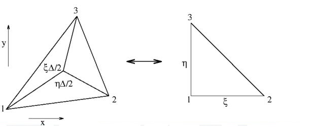
Thus $\xi$ can be interpreted as: area of the sub-triangle spanned by the
vectors $ (x - x_1 , y - y_1) $ and $ (x_3 - x_1 , y_3 - y_1) $
divided by the whole triangle area.
And $\eta$ can be interpreted as: area of the sub-triangle spanned by the
vectors $ (x - x_1 , y - y_1) $ and $ (x_2 - x_1 , y_2 - y_1) $
divided by the whole triangle area.
This is the reason why $ \xi $ and $ \eta $ are sometimes called
area-coordinates; see the above figure, where (two times) the area of the
triangle as a whole is denoted as $\Delta$.
There exist even three of these coordinates in literature. But
the third area-coordinate is, of course, dependent on the other two,
being equal to $(1-\xi-\eta)$.
Instead of area-coordinates, we prefer to talk about local coordinates
$\xi$ and $\eta$ of an element, in contrast to the global coordinates
$x$ and $y$.
It is possible that local coordinates coincide with the global coordinates.
A triangle for which such is the case is called a parent element.
The portrait of the parent triangle is also depicted in the above figure:
it is rectangular, and two sides of it are equal.
Let's reconsider the expression:
$$
T - T_1 = \xi .(T_2 - T_1) + \eta.(T_3 - T_1)
$$
Partial differentiation to $ \xi $ and $ \eta $ gives:
$$
\oq{T}{\xi} = T_2 - T_1 \quad ; \quad \oq{T}{\eta} = T_3 - T_1
$$
Therefore, with node (1) as the origin, hence $T(0)=T_1$:
$$
T = T(0) + \xi \dq{T}{\xi} + \eta \dq{T}{\eta}
$$
This is part of a Taylor series expansion around node (1). Such Taylor series
expansions are quite common in Finite Difference analysis.
Now rewrite as follows:
$$
T = (1 - \xi - \eta ).T_1 + \xi.T_2 + \eta.T_3
$$
Here the functions $ (1-\xi-\eta) , \, \xi , \, \eta $ are called the
shape functions of the Finite Element. Shape functions $N_k$ have the property
that they are unity in one of the nodes (k), and zero in all other nodes.
In our case:
$$
N_1 = 1-\xi-\eta \quad ; \quad N_2 = \xi \quad ; \quad N_3 = \eta
$$
So we have two representations, which are almost trivially equivalent:
$$ \begin{array}{ll}
T = T_1 + \xi.(T_2 - T_1) + \eta.(T_3 - T_1) \quad
& \mbox{: Finite Difference like} \\
T = (1 - \xi - \eta).T_1 + \xi.T_2 + \eta.T_3 \quad
& \mbox{: Finite Element like}
\end{array} $$
What kind of terms can be discretized at the domain of a linear triangle?
In the first place, the function $T(x,y)$ itself, of course. But one may also
try the first order partial derivatives $\oq{T}{x}$ , $\oq{T}{y}$. We find:
$$ \begin{array}{ll}
\oq{T}{x} = A = [ (y_3 - y_1).(T_2 - T_1) - (y_2 - y_1).(T_3 - T_1) ]/\Delta \\
\oq{T}{y} = B = [ (x_2 - x_1).(T_3 - T_1) - (x_3 - x_1).(T_2 - T_1) ]/\Delta
\end{array} $$
By collecting terms belonging to the same $T_k$, this can also be written as:
$$
\Delta \left[ \begin{array}{c} \oq{T}{x} \\ \oq{T}{y} \end{array} \right] =
\left[ \begin{array}{ccc} +(y_2 - y_3) & +(y_3 - y_1) & +(y_1 - y_2) \\
-(x_2 - x_3) & -(x_3 - x_1) & -(x_1 - x_2) \end{array}
\right] \left[ \begin{array}{c} T_1 \\ T_2 \\ T_3 \end{array} \right]
$$
Or, in operator form:
$$
\left[ \begin{array}{c} \oq{}{x} \\ \oq{}{y} \end{array} \right] =
\left[ \begin{array}{ccc} y_2 - y_3 & y_3 - y_1 & y_1 - y_2 \\
x_3 - x_2 & x_1 - x_3 & x_2 - x_1 \end{array}
\right] / \Delta $$
The right hand side will be called a Differentiation Matrix in subsequent
work. Thus the gradient operator at any linear triangle is represented by a
$2 \times 3$ differentiation matrix.