Second Order and Beyond for Multivariable Taylor Series
Least Squares Best Fit Methods are well known for a point, a straight
line, a circle, a conic section, in general: for a simple figure.
But that's not really cool. I'd rather have some least squares best fit
method with complicated figures, for example: two points, crossing
or parallel lines, a bunch of circles, the image of a character 'A'
- my ultimate dream being the least squares best fit with music score elements, a treble clef for example :-)
So far so good about dreams. But one has to start somewhere ..
Let's consider the most simple case (I think) in two dimensions: a least squares
best fit with two points instead of one. Writing the minimum principle
for this case is not too difficult.
Let the function M to be minimized be defined by:
$$
M(a,b,p,q) = \sum_k \left[ (x_k - a)^2 + (y_k - b)^2 \right].\left[ (x_k - p)^2 + (y_k - q)^2 \right]
$$
Here the $(x_k,y_k)$ are the fixed points of a cloud in the plane and we
are satisfied if we can find some fairly unique points $(a,b)$ and $(p,q)$ .
A procedure to accomplish this is rather straigtforward. Differentiate
the above sum to $\,(a,b,p,q)\,$ and put the four outcomes of these partial
differentiations equal to zero:
$$
F_a = \frac{\partial M(a,b,p,q)}{\partial a} = - 2 \sum_k (x_k - a)\left[ (x_k - p)^2 + (y_k - q)^2 \right] = 0\\
F_b = \frac{\partial M(a,b,p,q)}{\partial b} = - 2 \sum_k (x_k - b)\left[ (x_k - p)^2 + (y_k - q)^2 \right] = 0\\
F_p = \frac{\partial M(a,b,p,q)}{\partial p} = - 2 \sum_k (x_k - p)\left[ (x_k - a)^2 + (y_k - b)^2 \right] = 0\\
F_q = \frac{\partial M(a,b,p,q)}{\partial q} = - 2 \sum_k (x_k - q)\left[ (x_k - a)^2 + (y_k - b)^2 \right] = 0
$$
The next step is to employ a four dimensional
Newton-Raphson method to find the zeroes.
The one-dimensional equivalent is well known:
$$
x_{n+1} = x_n - \frac{F(x_n)}{F'(x_n)} \quad \Longleftrightarrow \quad F'(x_n)(x_{n+1}-x_n) = - F(x_n)
$$
It generalizes as follows ( with $\Delta x = x_{n+1}-x_n$ ) and mind the symmetry:
$$
\large \begin{bmatrix} \frac{\partial^2 M}{\partial a^2} & \frac{\partial^2 M}{\partial a \partial b}
& \frac{\partial^2 M}{\partial a \partial p} & \frac{\partial^2 M}{\partial a \partial q} \\
\frac{\partial^2 M}{\partial a \partial b} & \frac{\partial^2 M}{\partial b^2}
& \frac{\partial^2 M}{\partial b \partial p} & \frac{\partial^2 M}{\partial b \partial q} \\
\frac{\partial^2 M}{\partial a \partial p} & \frac{\partial^2 M}{\partial b \partial p}
& \frac{\partial^2 M}{\partial p^2} & \frac{\partial^2 M}{\partial p \partial q} \\
\frac{\partial^2 M}{\partial a \partial q} & \frac{\partial^2 M}{\partial b \partial q}
& \frac{\partial^2 M}{\partial p \partial q} & \frac{\partial^2 M}{\partial q^2} \end{bmatrix}_n
\begin{bmatrix} \Delta a \\ \Delta b \\ \Delta p \\ \Delta q \end{bmatrix} = - \begin{bmatrix} F_a \\ F_b \\ F_p \\ F_q \end{bmatrix}_n
$$
The matrix on the left is known as the Hessian matrix,
commonly denoted as $\,H$ . We need the inverse of it:
$$
H_n\,\Delta x = - F_n \quad \Longrightarrow \quad x_{n+1} = x_n - H_n^{-1}F_n
$$
So here are the OP's second order multivariable derivatives:
$$
\frac{\partial^2 M}{\partial a^2} = \frac{\partial^2 M}{\partial b^2} = 2 \sum_k \left[ (x_k - p)^2 + (y_k - q)^2 \right] \\
\frac{\partial^2 M}{\partial p^2} = \frac{\partial^2 M}{\partial q^2} = 2 \sum_k \left[ (x_k - a)^2 + (y_k - b)^2 \right] \\
\frac{\partial^2 M}{\partial a \partial p} = 4 \sum_k (x_k - a)(x_k - p) \qquad
\frac{\partial^2 M}{\partial a \partial q} = 4 \sum_k (x_k - a)(x_k - q) \\
\frac{\partial^2 M}{\partial b \partial p} = 4 \sum_k (x_k - b)(x_k - p) \qquad
\frac{\partial^2 M}{\partial b \partial q} = 4 \sum_k (x_k - b)(x_k - q) \\
\frac{\partial^2 M}{\partial a \partial b} = \frac{\partial^2 M}{\partial p \partial q} = 0
$$
Free software source implementing all this numerically and graphically is
found at my website .
It turns out that, given some neatly chosen conditions, iterations converge rather quickly to a result.
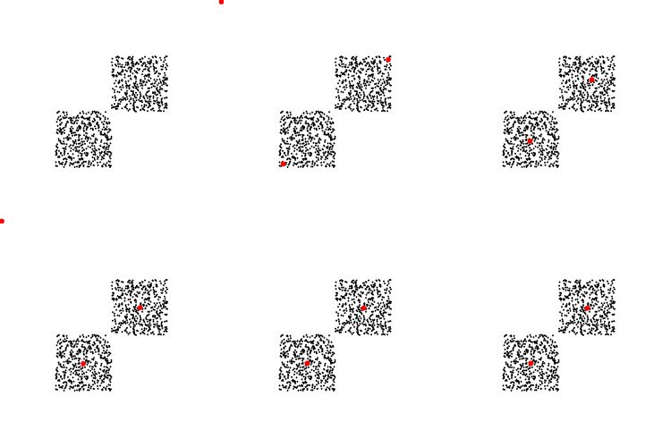
Here is an animation of $10$ iterations as generated by our software. The $\color{red}{\mbox{red dots}}$
correspond with the points $(a,b)$ and $(p,q)$ that are approaching to a best fit with the two squares of black dots.

Numerically:
( 0.030000000, 0.030000000)  ;  ( 3.970000000, 3.970000000)
( 0.660367766, 0.655184806)  ;  ( 3.346246442, 3.338009121)
( 1.067931194, 1.059662172)  ;  ( 2.947311493, 2.933165294)
( 1.224322703, 1.215456066)  ;  ( 2.610372656, 2.591778103)
( 1.483524248, 1.473141085)  ;  ( 2.587165222, 2.567701858)
( 1.492857336, 1.482684318)  ;  ( 2.507701174, 2.488004719)
( 1.500161598, 1.489958755)  ;  ( 2.505384218, 2.485704103)
( 1.500206864, 1.490003939)  ;  ( 2.505303084, 2.485623596)
( 1.500206877, 1.490003953)  ;  ( 2.505303074, 2.485623586)
( 1.500206877, 1.490003953)  ;  ( 2.505303074, 2.485623586)
The result of an observation of a function $\,f(x,y,z)\,$
with Gaussian blur $\,G(x,y,z)\,$ for example is
in general a convolution integral: $$ \overline{f} =
\iiint G(\xi,\eta,\zeta)\,f(x-\xi,y-\eta,z-\zeta)\,d\xi\,d\eta\,d\zeta $$
Here $\,G\,$ is the kernel function of the blur and $\,f\,$ is the function to be
observed. The function $\,f\,$ is developed into a Taylor series around
$\,(\xi,\eta,\zeta)=(0,0,0)$ :
$$ f(x-\xi,y-\eta,z-\zeta) \; \approx \; f(x,y,z) $$
$$ - \xi \frac{\partial f}{\partial x} - \eta \frac{\partial f}{\partial y} - \zeta \frac{\partial f}{\partial z} $$
$$ + \frac{1}{2} \xi^2 \frac{\partial^2 f}{\partial x^2} + \frac{1}{2} \eta^2 \frac{\partial^2 f}{\partial y^2}
+ \frac{1}{2} \zeta^2 \frac{\partial^2 f}{\partial z^2} $$
$$ + \xi \eta \frac{\partial f}{\partial x \partial y} + \eta \zeta \frac{\partial f}{\partial y \partial z}
+ \zeta \xi \frac{\partial f}{\partial z \partial x} $$
In this expression the partial differential quotients are no longer dependent
on $\,(\xi,\eta,\zeta)$ , because they are calculated for
$\,(\xi,\eta,\zeta)=(0,0,0)$ . Therefore the convolution integral is approximately
equal to:
$$ f(x,y,z) \iiint \, G \, d\xi\,d\eta\,d\zeta \\ \, - \, \frac{\partial f}{\partial x}
\iiint \xi \, G \, d\xi\,d\eta\,d\zeta \, - \, \frac{\partial f}{\partial y}
\iiint \eta \, G \, d\xi\,d\eta\,d\zeta \, - \, \frac{\partial f}{\partial z}
\iiint \zeta \, G \, d\xi\,d\eta\,d\zeta \\
+ \frac{1}{2} \frac{\partial^2 f}{\partial x^2}\iiint \xi^2 \, G \, d\xi\,d\eta\,\zeta
+ \frac{1}{2} \frac{\partial^2 f}{\partial y^2}\iiint \eta^2 \, G \, d\xi\,d\eta\,d\zeta
+ \frac{1}{2} \frac{\partial^2 f}{\partial z^2}\iiint \zeta^2\, G \, d\xi\,d\eta\,d\zeta \\
+ \frac{\partial f}{\partial x \partial y}\iiint \xi \eta \, G \, d\xi\,d\eta\,d\zeta
+ \frac{\partial f}{\partial y \partial z}\iiint \eta \zeta \, G \, d\xi\,d\eta\,d\zeta
+ \frac{\partial g}{\partial z \partial x}\iiint \zeta \xi \, G \, d\xi\,d\eta\,d\zeta
$$
The first integral is by definition equal to $\,1$ . The next three integrals are
equal to the expectation value of the Gaussian kernel function, and therefore equal
to $\,0$ . The next three integrals are equal to the spreads of the Gaussian kernel function
in the different coordinate directions. The last three integrals, at last, are
zero. Thus: $$ \overline{f} \approx
f + \frac{1}{2} \sigma_x^2 \frac{\partial^2 f}{\partial x^2} + \frac{1}{2} \sigma_y^2 \frac{\partial^2 f}{\partial y^2}
+ \frac{1}{2} \sigma_z^2 \frac{\partial^2 f}{\partial z^2} = f + \frac{1}{2} \sigma^2 \nabla^2 f $$
An asymptotic approximation for large distances, which can also be found
in any decent book about Statistics, where the last equality is for the
isotropic case only.
One possible application is the
renormalization
of singularities, for example the Electric field
of a point charge:
$$
E(r) = \frac{q}{4\pi\epsilon_0 r^2} \quad \mbox{with} \quad
\begin{cases} q = \mbox{(point) charge} \\ \epsilon_0 = \mbox{dielectric constant} \\ r = \mbox{distance to point} \end{cases}
$$
The far away field can be calculated without even knowing about the convolution integral:
$$
\overline{E} \approx E + \frac{1}{2} \sigma^2 \nabla^2 E \qquad \mbox{with} \qquad
\nabla^2 \frac{1}{r^2} =
\frac{1}{r} \frac{\partial^2}{\partial r^2} r \frac{1}{r^2} = \frac{2}{r^4}
$$
Hence:
$$
\overline{E} \approx E \left( 1 + \frac{\sigma^2}{r^2} \right) \quad \mbox{for} \quad r \gg \sigma
$$
The Electric field with Gaussian blur is:
$$
\overline{E}(x,y,z) = \left( \frac{1}{ \sigma \sqrt{2\pi} } \right)^3
\iiint \frac{q}{4 \pi \epsilon_0 ( \xi^2 + \eta^2 + \zeta^2 ) } \,
e^{\, - [ (\xi - x)^2 + (\eta - y)^2 + (\zeta - z)^2 ] / 2\sigma^2 }
\; d\xi\,d\eta\,d\zeta
$$
A special case is the value of the renormalized field at the origin, which turns out to be nicely finite :
$$
\overline{E}(r=0) = \left( \frac{1}{ \sigma \sqrt{2\pi} } \right)^3 \frac{q}{\epsilon_0}
\int_0^\infty e^{- r^2 / 2 \sigma^2 } d r =
\left( \frac{1}{ \sigma \sqrt{2\pi} } \right)^3 \frac{q}{\epsilon_0}
\frac{1}{2} \sigma \sqrt{2\pi} = \frac{q}{4 \pi \epsilon_0 \sigma^2 }
= E(\sigma)
$$
Anything in between is somewhat more difficult ..

