Theory is specified for a rectangular square lattice, therefore isoparametric transformations are out of order here.
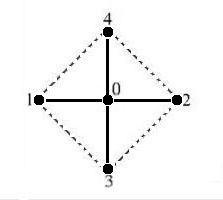
The above shape is known in Finite Difference circles as a five point star. Let its coordinates be given by: $$ (0) = (0,0) \quad ; \quad \begin{cases} (1) = (-1,0) \quad ; \quad (2) = (+1,0) \\ (3) = (0,-1) \quad ; \quad (4) = (0,+1)\end{cases} $$ Let function behaviour "inside" the five point star be approximated by a quadratic interpolation between the function values at the vertices or nodal points, let $T$ be such a function and use its Taylor expansion around the origin $(0)$: $$ T(x,y) = T(0) + \frac{\partial T}{\partial x}(0).x + \frac{\partial T}{\partial y}(0).y + \frac{1}{2} \frac{\partial^2 T}{\partial x^2}(0).x^2 + \frac{1}{2} \frac{\partial^2 T}{\partial y^2}(0).y^2 $$ Specify $T$ for the vertices with the basic polynomials of the five point star: $$ T_0 = T(0)\\ T_1 = T(0) - \frac{\partial T}{\partial x}(0) + \frac{1}{2} \frac{\partial^2 T}{\partial x^2}(0)\\ T_2 = T(0) + \frac{\partial T}{\partial x}(0) + \frac{1}{2} \frac{\partial^2 T}{\partial x^2}(0)\\ T_3 = T(0) - \frac{\partial T}{\partial y}(0) + \frac{1}{2} \frac{\partial^2 T}{\partial y^2}(0)\\ T_4 = T(0) + \frac{\partial T}{\partial y}(0) + \frac{1}{2} \frac{\partial^2 T}{\partial y^2}(0)\\ \quad \mbox{ F.E. } \leftarrow \mbox{ F.D. } $$ Solving these equations is not much of a problem and well-known Finite Difference schemes are recognized: $$ T(0) = T_0 \\ \frac{\partial T}{\partial x}(0) = \frac{T_2-T_1}{2}\\ \frac{\partial T}{\partial y}(0) = \frac{T_4-T_3}{2} \\ \frac{\partial^2 T}{\partial x^2}(0) = T_1-2T_0+T_2 \\ \frac{\partial^2 T}{\partial y^2}(0) = T_3-2T_0+T_4 \\ \quad \mbox{ F.D. } \leftarrow \mbox{ F.E. } $$ Finite Element shape functions may be constructed as follows: $$ T = N_0.T_0 + N_1.T_1 + N_2.T_2 + N_3.T_3 + N_4.T_4 = \\ T_0 + \frac{T_2-T_1}{2}x + \frac{T_4-T_3}{2}y + \frac{T_1-2T_0+T_2}{2}x^2 + \frac{T_3-2T_0+T_4}{2}y^2 =\\ (1-x^2-y^2)T_0 + \frac{1}{2}(-x+x^2)T_1 + \frac{1}{2}(+x+x^2)T_2 +\frac{1}{2}(-y+y^2)T_3 + \frac{1}{2}(+y+y^2)T_4 \\ \Longrightarrow \quad \begin{cases} N_0 = 1-x^2-y^2 \\ N_1 = (-x+x^2)/2\\ N_2 = (+x+x^2)/2\\ N_3 = (-y+y^2)/2\\ N_4 = (+y+y^2)/2 \end{cases} $$ So far so good concerning the generalities. Now specify for the problem at hand: $$ \frac{\partial T}{\partial x} = \frac{\partial T}{\partial x}(0)+\frac{\partial^2 T}{\partial x^2}(0).x = \frac{T_2-T_1}{2} + (T_1-2T_0+T_2).x = 0 \\ \Longrightarrow \quad x = - \frac{(T_2-T_1)/2}{T_1-2T_0+T_2} \\ \frac{\partial T}{\partial y} = \frac{\partial T}{\partial y}(0)+\frac{\partial^2 T}{\partial y^2}(0).y = \frac{T_4-T_3}{2} + (T_3-2T_0+T_4).y = 0 \\ \Longrightarrow \quad y = - \frac{(T_4-T_3)/2}{T_3-2T_0+T_4} $$ Substitute these $(x,y)$ values into either the F.D. or the F.E. formulation for $T(x,y)$ and you're done. The above can easily be generalized for multiple dimensions. As has been done in: