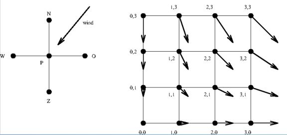
There are many roads to Rome. Talking about a given numerical velocity field, what do you mean? Among the many possibilities, there is a rectangular grid $(i,j)$ with velocities $(u,v)$ given at the vertices of the rectangles in the grid. Using ideal flow in a corner as the template, then we have for coordinates $(x,y)$ and velocities (see picture below): $$ x = i \quad ; \quad y = j \quad ; \quad u = x \quad ; \quad v = -y $$ The stream function $\psi(x,y)$ in general can be calculated with: $$ \color{red}{\frac{\partial \psi}{\partial x} = -v} \quad ; \quad \color{green}{\frac{\partial \psi}{\partial y} = +u} $$ Colors indicate that $\color{red}{horizontal}$ line segments shall be used for discretization of the first equation and $\color{green}{vertical}$ line segments shall be used for discretization of the second equation: $$ \color{red}{\psi_{i+1,j}-\psi_{i,j} = -j} \quad ; \quad \color{green}{\psi_{i,j+1}-\psi_{i,j} = +i} $$ Resulting in an overdetermined system of linear equations: $M$ equations with $N$ unknowns, where in our case
const
  grid : integer = 10;
  N := grid\*grid;
  M := 2\*(grid-1)\*grid;
The overdetermined equations are stored in a $M\times N$ matrix $\,A\,$ and a vector $\,r\,$ with length $M$ .
Now solve the equations $S\psi = b$ . Then what we get is a discretized stream function $\,\psi(x,y)$ .
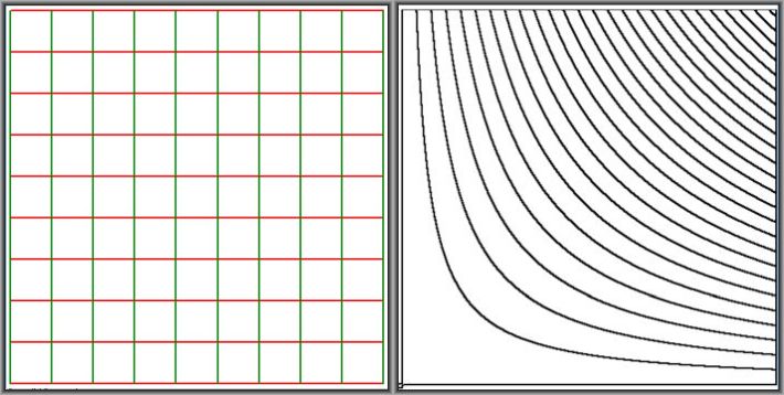
The isolines of $\,\psi\,$ are the streamlines and can be plotted as shown in the above picture on the right.
A bilinear interpolation at the rectangles in the grid is being employed for that purpose.
The software accomplishing all this is available for free, but it is far from optimal : take a look at
MSE publications / references in 2016 .
I hope you can generalize for your own purpose where such is needed. But again, there are many roads that lead to Rome,
especially in Numerical Analysis.
Update. In view of a comment by the OP:
$$
\color{red}{\frac{\partial \psi}{\partial x} = -v} \quad ; \quad \color{green}{\frac{\partial \psi}{\partial y} = +u}
\quad \Longrightarrow \\ d\psi = -v\,dx + u\,dy \quad \Longrightarrow \quad
\int_{(1)}^{(2)} d\psi = -\int_{(1)}^{(2)}v\, dx + \int_{(1)}^{(2)}u\, dy
\quad \Longrightarrow \\ \psi_2-\psi_1 \approx -\frac{v_1+v_2}{2}(x_2-x_1) + \frac{u_1+u_2}{2}(y_2-y_1) = (\vec{w_1}+\vec{w_2})/2 \times (\vec{r_2}-\vec{r_1})
$$
with $\,\vec{w} = (u,v)\,$ and $\,\vec{r} = (x,y)$ , interpreted physically as a discretized flux through a 1-D area.
An advantage of the latter formulation is that line segment( element)s no longer need to be vertical or horizontal.
This may be more appropriate with numerical methods that are Finite Element like.
Least Squares method. In case it needs a bit of explanation.
The system of overdetermined equations ($A\psi-r$) is squared, summed and minimized:
$$
(A\psi-r,A\psi-r) = \sum_{k=1}^M \left( \sum_{i=1}^N A_{ki} \psi_i - r_k \right)^2 = \,\operatorname{minimum}(\psi)
$$
By differentiating to $\,\psi_i\,$ we get $N$ (symmetric) equations with $N$ unknowns $S \psi = b$ :
$\partial/\partial \psi_i\, \operatorname{minimum}(\psi) =$
$$
2\sum_{k=1}^M A_{ki} \left( \sum_{j=1}^N A_{kj} \psi_j - r_k \right) = 0 \quad \Longrightarrow \\ \sum_{j=1}^N
\underbrace{\sum_{k=1}^M A_{ki} A_{kj}}_{\large S_{ij}}\, \psi_j = \underbrace{\sum_{k=1}^M A_{ki} r_k}_{\large b_i}
$$
Taking one step backwards, the integral form of the Least Squares (Finite Element) method is:
$$
\iint \left[\left(\frac{\partial \psi}{\partial x} + v \right)^2
+ \left(\frac{\partial \psi}{\partial y} - u \right)^2\right] dx\, dy = \mbox{minimum}(\psi)
$$
According to
calculus of variations
(or boldly differentiating to $\psi$ and discarding the integral signs):
$$
\frac{\partial}{\partial x}\left(\frac{\partial \psi}{\partial x} + v\right) +
\frac{\partial}{\partial y}\left(\frac{\partial \psi}{\partial y} - u\right) = 0
$$ $$
\frac{\partial^2 \psi}{\partial x^2} + \frac{\partial^2 \psi}{\partial y^2} =
- \omega \quad \mbox{with} \quad
\omega = \frac{\partial v}{\partial x} - \frac{\partial u}{\partial y}
$$
Which is recognized as Poisson's equation for the streamfunction, with vorticity on the right hand side.
This means that among the several roads to Rome there is a great chance that some of these are equivalent
with the method as presented in this answer. One advantage being that there is no numerical differentiation needed for calculating the vorticity.
Assembly. In the first answer, $M \times N$ overdetermined equations $A$ are defined first, where in our case $M = 180$ and $N = 100$. While forming the system matrix $S=A^TA$ we thus have $180\times 100^2$ operations, which is ridiculous because $A$ is almost empty: only $2$ of the $100$ entries in a row are non-zero! It's easy to improve this by defining $A$ as being an $1 \times 2$ array and forming $A^TA$ as an elementary matrix $E$, corresponding with just one equation; $r$ is the right hand side of it. $$ E = A^TA = \begin{bmatrix} -1 \\ +1 \end{bmatrix} \begin{bmatrix} -1 & +1 \end{bmatrix} = \begin{bmatrix} +1 & -1 \\ -1 & +1 \end{bmatrix} \\ r = \begin{bmatrix} -1 \\ +1 \end{bmatrix}\left[-v_{12}(x_2-x_1) + u_{12}(y_2-y_1)\right] $$ The elementary matrices $E$ and loads $r$ must subsequently be assembled into the system matrix $S$ and global load vector $b$. Which happens to be exactly the same procedure as is common with the conventional finite element method. The name Least Squares Finite Element Method is justified herewith.
Solving. Instead of defining a full $100\times 100$ system matrix $S$, it's far more efficient to define it as a band matrix. That will save us a factor $10$ of space in the first place. But there are a few other properties that are interesting: $$ \begin{cases} S_{ij} = \sum_k A_{ki}A_{kj} \quad \Longrightarrow \quad S_{ij}=S_{ji} \\ S_{ii} = \sum_k A_{ki}A_{ki} \quad \Longrightarrow \quad S_{ii} > 0 \\ \left(\sum_k A_{ki}A_{kj}\right)^2 \le \sum_k A_{ki}^2\cdot\sum_k A_{kj}^2 \quad \Longrightarrow \quad \left| S_{ij}\right| \le \sqrt{S_{ii} S_{jj}} \end{cases} $$ The last property by Schwarz inequality. Symmetry will save us another factor $2$ in space, but more importantly, the computation time for solving the equations will be reduced with a factor $100$ or so. The last two properties show that the system matrix $S$ is positive definite and diagonally dominant, meaning that all pivots are on the main diagonal.
All of the improvements have been implemented in the updated version of the software, labeled as "Second answer" of the question in MSE publications / references 2016.
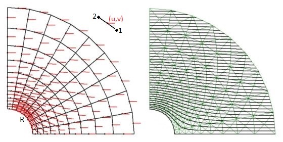
There is still another issue with the streamline (= streamfunction isoline) plot, as shown in the above picture on the right. Solving for the parameters of a Quadrilateral Interpolation, as would be needed with the algorithm for defining an isoline plot, is virtually impossible with quadrilaterals that are not paralellograms. Therefore we have subdivided each of our quads into four triangles. Thanks to an algorithm by Paul Bourke, defining isolines with triangles is a matter of routine.
The end-result is shown in the above picture on the right. Needless to say that there is a match with the exact solution for the streamline function.