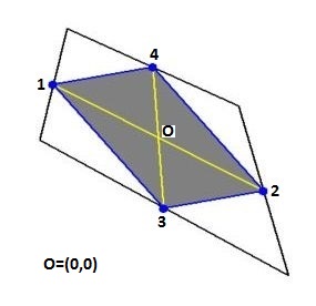
Any employment for the Varignon parallelogram?
The midpoints of the sides of an arbitrary quadrilateral form a parallelogram, which is called the
Varignon parallelogram of the quad.
While answering a question about
Quadrilateral Interpolation it has been found
that the Varignon parallelogram may be considered as a Finite Difference five point star in disguise. Moreover it has been
derived that the associated Finite Element interpolation for an arbitrary function $T$ inside the parallelogram is linear:
$$
T(\xi,\eta) = T(0,0) + \frac{\partial T}{\partial \xi}(0,0).\xi
+ \frac{\partial T}{\partial \eta}(0,0).\eta
$$
with $-1 < \xi+\eta < +1$ and $-1 < \xi-\eta < +1$ and:
$$
T(0,0) = \frac{T_1+T_2}{2}=\frac{T_3+T_4}{2}\\
\frac{\partial T}{\partial \xi}(0,0) = \frac{T_2-T_1}{2}\\
\frac{\partial T}{\partial \eta}(0,0) = \frac{T_4-T_3}{2}
$$
The local parameters $(\xi,\eta)$ can be expressed in the global $(x,y)$ coordinates via:
$$
\begin{bmatrix} \xi \\ \eta \end{bmatrix} =
\begin{bmatrix} (x_2-x_1)/2 & (x_4-x_3)/2 \\ (y_2-y_1)/2 & (y_4-y_3)/2 \end{bmatrix}^{-1}
\begin{bmatrix} x-x(0,0) \\ y-y(0,0) \end{bmatrix} \\ \mbox{with} \quad
\begin{cases} x(0,0) = (x_1+x_2)/2=(x_3+x_4)/2\\y(0,0) = (y_1+y_2)/2=(y_3+y_4)/2\end{cases}
$$
It all seems like the Varignon parallelogram may be employable, for example as as a suitable Finite Element.
But I haven't seen yet any applications for it in printed mathematical literature.
The applications I am
looking for are not required to be numerical in nature, though. I'm curious to see anything of practical use.
Update. Talking about Finite Element applications, let us consider the (global) partial derivatives
of an arbitrary function $T$ at the parallelogram : $\partial T/\partial x\,$ and $\,\partial T/\partial y$ .
Like in the answer
here
it is advantageous to start the other way around:
$$
\frac{\partial T}{\partial \xi} =
\frac{\partial T}{\partial x}\frac{\partial x}{\partial \xi}
+\frac{\partial T}{\partial y}\frac{\partial y}{\partial \xi} \\
\frac{\partial T}{\partial \eta} =
\frac{\partial T}{\partial x}\frac{\partial x}{\partial \eta}
+\frac{\partial T}{\partial y}\frac{\partial y}{\partial \eta}
$$
The matrix formulation of this clearly shows that the inverse is what we need:
$$ \Large
\begin{bmatrix} \frac{\partial T}{\partial \xi} \\ \frac{\partial T}{\partial \eta} \end{bmatrix} =
\begin{bmatrix} \frac{\partial x}{\partial \xi} & \frac{\partial y}{\partial \xi} \\
\frac{\partial x}{\partial \eta} & \frac{\partial y}{\partial \eta} \end{bmatrix}
\begin{bmatrix} \frac{\partial T}{\partial x} \\ \frac{\partial T}{\partial y} \end{bmatrix}
\quad \Longleftrightarrow \\ \Large
\begin{bmatrix} \frac{\partial T}{\partial x} \\ \frac{\partial T}{\partial y} \end{bmatrix} =
\begin{bmatrix} \frac{\partial x}{\partial \xi} & \frac{\partial y}{\partial \xi} \\
\frac{\partial x}{\partial \eta} & \frac{\partial y}{\partial \eta} \end{bmatrix}^{-1}
\begin{bmatrix} \frac{\partial T}{\partial \xi} \\ \frac{\partial T}{\partial \eta} \end{bmatrix} =
\begin{bmatrix} \frac{\partial y}{\partial \eta} & -\frac{\partial y}{\partial \xi} \\
-\frac{\partial x}{\partial \eta} & \frac{\partial x}{\partial \xi} \end{bmatrix} / \Delta
\begin{bmatrix} \frac{\partial T}{\partial \xi} \\ \frac{\partial T}{\partial \eta} \end{bmatrix}
$$ $$
\mbox{with} \quad \Delta =
\frac{\partial x}{\partial \xi} \frac{\partial y}{\partial \eta} -
\frac{\partial x}{\partial \eta} \frac{\partial y}{\partial \xi}
$$
The rest is easy, because:
$$
\frac{\partial x}{\partial \xi} = \frac{x_2-x_1}{2}\quad ; \quad
\frac{\partial y}{\partial \xi} = \frac{y_2-y_1}{2}\quad ; \quad
\frac{\partial T}{\partial \xi} = \frac{T_2-T_1}{2}\\
\frac{\partial x}{\partial \eta} = \frac{x_4-x_3}{2}\quad ; \quad
\frac{\partial y}{\partial \eta} = \frac{y_4-y_3}{2}\quad ; \quad
\frac{\partial T}{\partial \eta} = \frac{T_4-T_3}{2}
$$
But okay, for the sake of completeness:
$$
\frac{\partial T}{\partial x} = \frac{(T_2-T_1)(y_4-y_3)-(T_4-T_3)(y_2-y_1)}{(x_2-x_1)(y_4-y_3)-(x_4-x_3)(y_2-y_1)}\\
\frac{\partial T}{\partial y} = \frac{(x_2-x_1)(T_4-T_3)-(x_4-x_3)(T_2-T_1)}{(x_2-x_1)(y_4-y_3)-(x_4-x_3)(y_2-y_1)}
$$
Cramer's rule is clearly recognized herein.
Discretizations for Ideal Flow
at the Varignon parallelogram
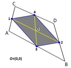
Quadrilateral vertex coordinates, as observed (with Microsoft Paint) in the $285 \times 276$ picture:
$$
\vec{A} = (36,276-126) \quad ; \quad \vec{B} = (259,276-247) \\
\vec{C} = (61,276-25) \quad ; \quad \vec{D} = (215,276-95)
$$
Coordinates of the Varignon parallelogram, accordingly:
$$
(x_1,y_1) = \frac{\vec{A}+\vec{C}}{2} \quad ; \quad (x_2,y_2) = \frac{\vec{B}+\vec{D}}{2}
\quad ; \quad (x_3,y_3) = \frac{\vec{A}+\vec{B}}{2} \quad ; \quad (x_4,y_4) = \frac{\vec{C}+\vec{D}}{2}
$$
Equations of ideal flow ,
with $(u,v) = $ velocities and $(x,y) = $ Cartesian coordinates:
$$
\frac{\partial u}{\partial x} + \frac{\partial v}{\partial y} = 0 \quad \mbox{: incompressible} \quad ; \quad
\frac{\partial v}{\partial x} - \frac{\partial u}{\partial y} = 0 \quad \mbox{: irrotational}
$$
Green's Theorem :
$$
\underbrace{\iint_D \left(\frac{\partial Q}{\partial x} - \frac{\partial P}{\partial y}\right)dx\,dy}_\mbox{Finite Element Method} \quad =
\underbrace{\oint_{\partial D} \left(P\,dx + Q\,dy\right)}_\mbox{Finite Volume Method}
$$
Applied to ideal flow:
$$
\iint_D \left(\frac{\partial u}{\partial x} + \frac{\partial v}{\partial y}\right)dx\,dy =
\oint_{\partial D} \left(u\,dy - v\,dx\right) = 0\\
\iint_D \left(\frac{\partial v}{\partial x} - \frac{\partial u}{\partial y}\right)dx\,dy =
\oint_{\partial D} \left(u\,dx+v\,dy\right) = 0
$$
Discretization of velocities at the vertices of the Varignon parallelogram:
$$
\vec{w} = (u_1,v_1) , (u_2,v_2) , (u_3,v_3) , (u_4,v_4)
$$
Discretization of the area of the Varignon parallelogram:
$$
\det\left(\vec{12},\vec{34}\right) = \det\left(\vec{13}+\vec{32},\vec{32}+\vec{24}\right) = \\
\det\left(\vec{13},\vec{32}\right)+\det\left(\vec{13},\vec{24}\right)+\det\left(\vec{32},\vec{32}\right)+\det\left(\vec{32},\vec{24}\right) = \\
\mbox{area} + 0 + 0 + \mbox{area} \quad \Longrightarrow \\
\mbox{area} = \frac{1}{2} \left[(x_2-x_1)(y_4-y_3)-(x_4-x_3)(y_2-y_1)\right]
$$
Discretization of incompressible flow left hand side integral with help of FEM partial derivatives for the function $T$ - see
question - and the area:
$$
\iint_D \left(\frac{\partial u}{\partial x} + \frac{\partial v}{\partial y}\right)dx\,dy = \frac{1}{2} \times \\
\left[(u_2-u_1)(y_4-y_3)-(u_4-u_3)(y_2-y_1)\right] + \left[(x_2-x_1)(v_4-v_3)-(x_4-x_3)(v_2-v_1)\right]
$$
Discretization of irrotational flow left hand side integral with help of FEM partial derivatives for the function $T$ - see
question - and the area:
$$
\iint_D \left(\frac{\partial v}{\partial x} - \frac{\partial u}{\partial y}\right)dx\,dy = \frac{1}{2} \times \\
\left[(v_2-v_1)(y_4-y_3)-(v_4-v_3)(y_2-y_1)\right] - \left[(x_2-x_1)(u_4-u_3)-(x_4-x_3)(u_2-u_1)\right]
$$
Discretization of line segments:
$$
(dx,dy) = (x_3-x_1,y_3-y_1) , (x_2-x_3,y_2-y_3) , (x_4-x_2,y_4-y_2) , (x_1-x_4,y_1-y_4)
$$
Discretization of velocities at line segments:
$$
\vec{w} = (u_3+u_1,v_3+v_1)/2 , (u_2+u_3,v_2+v_3)/2 , (u_4+u_2,v_4+v_2)/2 , (u_1+u_4,v_1+v_4)/2
$$
Discretization of incompressible flow FVM right hand side integral:
$$
\oint_{\partial D} \left(u\,dy - v\,dx\right) = \\
\left[(u_3+u_1)/2\,(y_3-y_1)-(v_3+v_1)/2\,(x_3-x_1)\right] + \left[(u_1+u_4)/2\,(y_1-y_4)-(v_1+v_4)/2\,(x_1-x_4)\right] \\
+ \left[(u_4+u_2)/2\,(y_4-y_2)-(v_4+v_2)/2\,(x_4-x_2)\right] + \left[(u_2+u_3)/2\,(y_2-y_3)-(v_2+v_3)/2\,(x_2-x_3)\right] = \\
\frac{1}{2}\left[(u_2-u_1)(y_4-y_3)-(u_4-u_3)(y_2-y_1)-(v_2-v_1)(x_4-x_3)+(v_4-v_3)(x_2-x_1)\right]
$$
Which is identical to the discretization of the incompressible flow FEM left hand side integral.
Discretization of irrotational flow FVM right hand side integral:
$$
\oint_{\partial D} \left(u\,dx+v\,dy\right) = \\
\left[(u_3+u_1)/2\,(x_3-x_1)+(v_3+v_1)/2\,(y_3-y_1)\right] + \left[(u_1+u_4)/2\,(x_1-x_4)+(v_1+v_4)/2\,(y_1-y_4)\right] \\
+ \left[(u_4+u_2)/2\,(x_4-x_2)+(v_4+v_2)/2\,(y_4-y_2)\right] + \left[(u_2+u_3)/2\,(x_2-x_3)+(v_2+v_3)/2\,(y_2-y_3)\right] = \\
\frac{1}{2}\left[(u_2-u_1)(x_4-x_3)-(u_4-u_3)(x_2-x_1)+(v_2-v_1)(y_4-y_3)-(v_4-v_3)(y_2-y_1)\right]
$$
Which is identical to the discretization of the irrotational flow FEM left hand side integral.
It's not trivial that the proposed FEM and FVM discretizations are identical & consistent with Green's theorem .
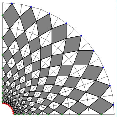
The $9\times 9$ computational grid with Varignon parallelograms is shown.
Boundary conditions are as follows:
$$
\begin{cases}
\color{red}{\mbox{inner circle impermeable:}} & (\vec{w}\cdot\vec{AB}) = 0 \\
\color{blue}{\mbox{outer circle uniform flow:}} & u = 1 \\
\color{green}{\mbox{inflow opening left:}} & v = 0 \\
\color{green}{\mbox{line of symmetry bottom:}} & v = 0 \end{cases}
$$
The curvilinear grid is topologically equivalent with a $\mbox{NDX}\times\mbox{NDY}$ rectangular grid (with $\mbox{NDX}=\mbox{NDY}=9$).
Let's make a count of the unknowns and the equations and see if there is a match. First the unknowns:
$$
\mbox{# velocities } (u,v) = 2\times\left[\mbox{NDX}(\mbox{NDY}+1)+\mbox{NDY}(\mbox{NDX}+1)\right] \quad \Longrightarrow \\
\mbox{# unknowns} = 4\times\mbox{NDX}\times\mbox{NDY}+2\times\mbox{NDX}+2\times\mbox{NDY}
$$
Second the equations:
$$\begin{cases}
\mbox{# incompressible + irrotational} = 2\times \mbox{NDX}\times\mbox{NDY} \\
\mbox{# boundary conditions} = 2\times \left[\mbox{NDX}+\mbox{NDY}\right]\end{cases} \quad \Longrightarrow \\
\mbox{# equations} = 2\times\mbox{NDX}\times\mbox{NDY}+2\times\mbox{NDX}+2\times\mbox{NDY}
$$
Therefore $2\times\mbox{NDX}\times\mbox{NDY}$ equations are missing. Did we forget something? Yes we did!
Remember the coordinates of the Varignon parallelogram:
$$
(x_1,y_1) = \frac{\vec{A}+\vec{C}}{2} \quad ; \quad (x_2,y_2) = \frac{\vec{B}+\vec{D}}{2}
\quad ; \quad (x_3,y_3) = \frac{\vec{A}+\vec{B}}{2} \quad ; \quad (x_4,y_4) = \frac{\vec{C}+\vec{D}}{2}
$$
However, the above does not hold only for the coordinates; it holds for any function $T$ at the parallelogram.
This phenomenon is known in Finite Element circles as isoparametrics:
$$
T_1 = \frac{T_A+T_C}{2} \quad ; \quad T_2 = \frac{T_B+T_D}{2}
\quad ; \quad T_3 = \frac{T_A+T_B}{2} \quad ; \quad T_4 = \frac{T_C+T_D}{2}
$$
Herefrom we easily conclude, quite in general:
$$
\frac{T_A+T_B+T_C+T_D}{2} = T_1 + T_2 = T_3 + T_4
$$
for any function $T$, in particular for the coordinates, but also for the velocity components $(u,v)$ :
$$
u_1 + u_2 = u_3 + u_4 \quad ; \quad v_1 + v_2 = v_3 + v_4
$$
So here we are! The isoparametrics is giving us exactly the $2\times\mbox{NDX}\times\mbox{NDY}$ equations that we were missing.
We end up with $N$ independent linear equations with $N$ unknowns (: $N = 360$).
A system that can be solved, in principle.
There is one little problem, however. With many Finite Difference discretizations, the resulting linear system is
such that one can tell which equation belongs to which unknown. But our system is such that it is impossible to
order them according to the unknowns. It is for this reason that a somewhat indirect solution method may be preferred:
Least Squares. I'm not going to explain this method again and again. Relevant MSE references:
Last but not least, free (Delphi Pascal) source code is available as:
Needless to say that the numerical results of the program are in close (enough) agreement with the analytical solution?