Laplace transform for dummies
Maybe the heuristics below is for smarties rather than for dummies, but anyway here goes.
For the sake of rigor: assuming that all (improper) integrals exist and everything is real-valued.
The Taylor series expansion of a function $ f(t+\tau) $ around $ t $ will be set up:
$$
f(t+\tau) = \sum_{k=0}^\infty \frac{ \tau^k }{ k ! } f^{(k)}(t)
= \left[ \sum_{k=0}^\infty \frac{1}{k!}
\left( \tau \ \frac{d}{dt} \right)^k \right] f(t)
$$
In the expression between square brackets the series expansion of $\,e^x\,$ is
recognized. Therefore we can write , symbolically :
$$
f(t+\tau) = e^{\Large \tau \frac{d}{dt} } f(t) \quad \Longrightarrow \quad
f(t-\tau) = e^{\Large -\tau \frac{d}{dt} } f(t)
$$
With the last formula in mind, consider an arbitrary convolution-integral:
$$
\int_{-\infty}^{+\infty} h(\tau) f(t-\tau) \, d\tau
$$
Convolution integrals do frequently occur. With a linear system, the response at
a disturbance is the convolution-integral of the disturbance with the so-called
(impulse) response.
The unit response is the way in which the system reacts upon the simplest of all
disturbances, that is a steep peak of very short duration at time zero, a
Dirac delta.
Our convolution integral can be rewritten with help of the expression for $ f(t-\tau) $ as follows:
$$
= \int_{-\infty}^{+\infty} h(\tau) \left[e^{\Large - \tau \frac{d}{dt} } f(t) \right]\, d\tau =
\int_{-\infty}^{+\infty} h(\tau) e^{\Large - \tau \frac{d}{dt} } \, d\tau \; \cdot \; f(t)
$$
The integral on the right should be well known to us. Quite "incidentally"
namely it is the (double-sided) Laplace transform:
$$
H(p) = \int_{-\infty}^{+\infty} e^{\large - p \tau}\, h(\tau) \, d\tau
$$
Thus it seems that Laplace's integral shows up quite spontaneously with elementary
considerations about convolution-integrals in combination with
Operational
Calculus . The end-result is:
$$
\int_{-\infty}^{+\infty} h(\tau) f(t-\tau) \, d\tau = H(\frac{d}{dt}) \, f(t)
$$
The fact that Laplace transforms are a very powerful means for solving differential
equations can now be understood without much effort. Suppose we have a linear
inhomogeneous differential equation. In general it has the form:
$$
D( \frac{d}{dt} ) \, \phi(t) = f(t)
$$
Then with help of our
Operator/Operational Calculus we can immediately write the solution as:
$$
\phi(t) = \frac{1}{\large D( \frac{d}{dt} ) } f(t)
$$
Put $\,H(d/dt) = 1/D(d/dt) $ , then the excercise becomes: find the inverse
of the Laplace transform of $\, H(p) $ . Call this inverse function $\, h(t) $ .
Finding the solution then follows the above pattern:
$$
\phi(t) = \int_{-\infty}^{+\infty} h(\tau) f(t-\tau) \, d\tau
$$
Example 1. Suppose that we have derived (for $p>\alpha$):
$$
h(t) = e^{\large \alpha t}.u(t) \quad \Longrightarrow \quad H(p) =
\int_{-\infty}^{+\infty} e^{\large -p\tau} e^{\large \alpha \tau}.u(\tau) d\tau =\\
\int_0^\infty e^{\large -p\tau} e^{\large \alpha \tau} d\tau =
\left[\frac{-e^{\large -\tau(p-\alpha)}}{p-\alpha}\right]_{\tau=0}^\infty =
\frac{1}{p-\alpha}
$$
Where the Heaviside step function $u(t)$ is defined by:
$$ u(t) =
\begin{cases} 0 & \mbox{for} & t < 0\\ 1 & \mbox{for} & t > 0\end{cases}
$$
Now consider the differential equation:
$$
\frac{d\phi}{dt} + \phi(t) = 0 \quad \mbox{with} \quad \phi(0)=1
$$
Which safely can be replaced by finding a
Green's function in the time domain:
$$
\frac{d\phi}{dt} + \phi(t) = \delta(t) \quad \mbox{with} \quad \phi(-\infty)=0
$$
It follows that:
$$
\phi(t) = \frac{1}{\large \frac{d}{dt} + 1 } =
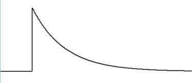
\int_{-\infty}^{+\infty} e^{\large - \tau}.u(\tau) \delta(t-\tau) \, d\tau = e^{\large - t}.u(t)
$$
Example 2. Still with us? Then let's investigate the Laplace transform of
$\,\exp(-\mu t^2)$ :
$$
\int_{-\infty}^{+\infty} e^{-pt} e^{-\mu t^2} \, dt = \int_{-\infty}^{+\infty} e^{-\mu t^2-pt}\, dt
$$
Completing the square $\;\mu t^2 + pt= \mu\left[t^2+p/\mu.t+p^2/(2\mu)^2\right]-p^2/4\mu = x^2-p^2/4\mu\;$ with $\,x = t + p/2\mu\,$ results in:
$$
= \int_{-\infty}^{+\infty} e^{-\mu x^2} \, dx \,.\, e^{\,p^2/4\mu }
= \sqrt{ \frac{\pi}{\mu} } e^{\,p^2 / 4\mu }
$$
The last move by using a well-known result for the integral of the
Gaussian probability distribution.
Laplace transform $H$ and inverse Laplace transform $h$ are thus mutually related as follows, after having replaced $1/4\mu$ by $1/2\sigma^2$ :
$$
H(p) = e^{\, \frac{1}{2} \sigma^2 p^2 } \quad \Longleftrightarrow \quad
h(t) = \frac{1}{ \sigma \sqrt{2\pi} } e^{-t^2 / 2\sigma^2 }
$$
A convolution integral with the normal distribution $h(t)$ as the kernel can thus be re-written as:
$$
\int_{- \infty}^{+ \infty} \! h(\xi) \phi(x-\xi) \, d\xi =
e^{\frac{1}{2} \sigma^2 \frac{d^2}{dx^2} } \phi(x)
$$
The physical meaning of this is that the (Gaussian blur)
operator $\,\exp(\frac{1}{2} \sigma^2 \large \frac{d^2}{dx^2})\,$ "spreads out" the function $\,\phi(x)\,$ over a domain with size of the order $\,\sigma $ .
The above outcome is immediately applicable to the following problem. Let's consider
the (partial differential) equation
for diffusion of heat in one-dimensional space and time:
$$
\frac{\partial T}{\partial t} = a \frac{\partial^2 T}{\partial x^2}
$$
Here $x=$ space, $t=$ time, $T=$ temperature, $a=$ constant. Rewrite in the first place as follows:
$$
\lambda \frac{\partial}{\partial t} T = \lambda a \frac{\partial^2}{\partial x^2} T
$$
As a next step we exponentiate at both sides the operators in place:
$$
e^{\lambda \partial/\partial t } \, T = e^{\lambda a \partial^2 / \partial x^2} \, T
$$
The resulting operator-expressions can be converted into classical
mathematics with the acquired knowledge:
$$
T(x,t+\lambda) = \int_{- \infty}^{+ \infty} \! h(\xi) T(x-\xi,t) \, d\xi
$$
Where $ \frac{1}{2} \sigma^2 = \lambda a $. Therefore:
$$
h(t) = \frac{1}{ \sigma \sqrt{2\pi} } \, e^{-t^2/2\sigma^2 } \quad \to \quad
h(\xi) = \frac{1}{ \sqrt{4\pi \lambda a} } \, e^{-\xi^2/(4\lambda a) }
$$
At last exchange $t$ and $\lambda$, and substitute $\lambda = 0$. Then we quickly find the solution of our PDE:
$$
T(x,t) = \int_{- \infty}^{+ \infty} \!
\frac{1}{\sqrt{4\pi a t}}\, e^{- \xi^2/(4 a t) }\, T(x-\xi,0) \, d\xi
$$