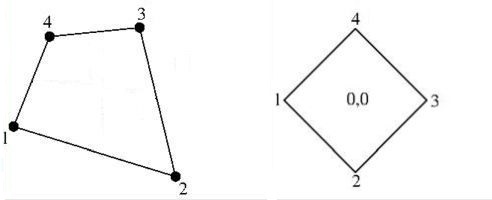
But now we have a little problem. Consider the quadrilateral as depicted in the above picture on the right. The vertex-coordinates of this quadrilateral are defined by the second and the third column of the matrix below. This matrix is formed by specifying $T$ vertically for the nodal points and horizontally for the basic functions $ 1,x,y,xy $ : $$ \begin{bmatrix} T_1 \\ T_2 \\ T_3 \\ T_4 \end{bmatrix} = \begin{bmatrix} 1 & -\frac{1}{2} & 0 & 0 \\ 1 & 0 & -\frac{1}{2} & 0 \\ 1 & +\frac{1}{2} & 0 & 0 \\ 1 & 0 & +\frac{1}{2} & 0 \end{bmatrix} \begin{bmatrix} A \\ B \\ C \\ D \end{bmatrix} $$ The last column of the matrix is zero. Hence it is singular, meaning that $A,B,C$ and $D$ cannot be found in this manner. Though with a unstructured grid there may seem to be not a great chance that a quadrilateral is exactly positioned like this, experience reveals that it cannot be excluded that Murphy comes by. That alone is enough reason to declare the method for triangles not done for quadrilaterals.
Two questions:
EDIT. The comment by Rahul sheds some light. Let the finite element shape be "modified" by an affine transformation (with $a,b,c,d,p,q$ arbitrary real constants) and work out for the term that is interesting: $$\begin{cases} x' = ax+by+p \\ y' = cx+dy+q \end{cases} \quad \Longrightarrow \\ x'y'=acx^2+bdy^2 + (ad+bc)xy+(cp+aq)x+(dp+bq)y+pq $$ So the interpolation remains bilinear only when the following conditions are fulfilled: $$ ac=0 \; \wedge \; bd=0 \; \wedge \; ad+bc\ne 0 \quad \Longleftrightarrow \\ \begin{cases} a\ne 0 \; \wedge \; d\ne 0 \; \wedge \; b=0 \; \wedge \; c=0 \\ a=0 \; \wedge \; d=0 \; \wedge \; b\ne 0 \; \wedge \; c\ne 0 \end{cases}\quad \Longleftrightarrow \\ \begin{cases}x'=ax+p\\y'=dy+q\end{cases} \quad \vee \quad \begin{cases}x'=by+p\\y'=cx+q\end{cases} $$ This means that a (parent) quadrilateral element, once it has been chosen, can only be translated, scaled (in $x$- and/or $y$- direction), mirrored in $\,y=\pm x$ , rotated over $90^o$. Did I forget something?
Update.
Why a quadrilateral with bilinear interpolation?
Little else is possible with polynomial terms like $\;1,\xi,\eta,\xi\eta\,$ , if four nodal points are needed (one degree of freedom each) for obtaining four equations with four unknowns. Then stil there remain some issues, such as not self-intersecting and being convex. The former issue has been covered in the answer by Nominal Animal. The latter may be stuff for a separate question.
Other issues covered in the answer by Nominal Animal are the following.
- Perhaps the simplest heuristics is to take the direct product of one-dimensional case: the line segment as well as the linear interpolation. With the notations by Rahul and Nominal Animal that is: $[0,1]\times[0,1]$ and $\{1,u\}\times\{1,v\}$ . In the end, we have a square as the standard parent bilinear quadrilateral. - For a non-degenerate paralellogram the bilinear interpolation is reduced to a linear one, which makes it simple to express the local coordinates $(u,v)$ into the global coordinates $(x,y)$.
LATE EDIT. Continuing story at:
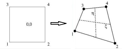
The parent element that will be adopted for
our own purpose is not quite the unit square. Instead it is:
$\,[-1,+1]\times[-1,+1]$ . And the local coordinates inside our parent quadrilateral
are defined accordingly: $\,-1 \leq \xi \leq +1\,$ and $\,-1 \leq \eta \leq +1\,$ . It's
the same material as employed by Rahul and Nominal Animal if we only substitute
$\,\xi = 2u-1$ and $\eta = 2v-1\;$ i.e. translation and scaling of the same shape
(see the question's EDIT). The node numbering as proposed by Nominal Animal
has been implemented here as follows: $\,\operatorname{nr}(x,y) = 2y+x+1\,$
with $\,x \in \{0,1\}\,$ and $\,y \in \{0,1\}$ .
The advantage being that, in contrast with the more common counterclockwise convention,
such a numbering can be generalized smoothly to three dimensions and higher.
Okay, whatever. Let function behaviour inside a FEM quadrilateral be approximated
by a bilinear interpolation between the function values at the vertices or nodal points, let $T$ be such a function:
$$
T = A_T + B_T.\xi + C_T.\eta + D_T.\xi.\eta
$$
It is assumed that the same parameters $(\xi,\eta)$ are employed for the function
$T$ as well as for the (global Cartesian) coordinates $x$ and $y$. Herewith it is
expressed that we have, as with the linear triangle, an isoparametric transformation:
$$
x = A_x + B_x.\xi + C_x.\eta + D_x.\xi.\eta \\
y = A_y + B_y.\xi + C_y.\eta + D_y.\xi.\eta
$$
Now specify any function $T$ for the vertices and the basic functions:
$$
\begin{bmatrix} T_1 \\ T_2 \\ T_3 \\ T_4 \end{bmatrix} =
\begin{bmatrix} +1 & -1 & -1 & +1 \\
+1 & +1 & -1 & -1 \\
+1 & -1 & +1 & -1 \\
+1 & +1 & +1 & +1 \end{bmatrix}
\begin{bmatrix} A_T \\ B_T \\ C_T \\ D_T \end{bmatrix}
\quad \mbox{ F.E } \leftarrow \mbox{ F.D. }
$$
It is remarked that the above matrix is orthogonal, i.e. its columns are
mutually perpendicular. This also means that the "condition" of the matrix is
optimal. Even better, it is similar to the well-known $4\times 4$
Hadamard matrix.
Apart from a scaling factor $4$, the inverse matrix is equal to the transpose,
which can be determined easily:
$$
\begin{bmatrix} A_T \\ B_T \\ C_T \\ D_T \end{bmatrix} = \frac{1}{4}
\begin{bmatrix} +1 & +1 & +1 & +1 \\
-1 & +1 & -1 & +1 \\
-1 & -1 & +1 & +1 \\
+1 & -1 & -1 & +1 \end{bmatrix}
\begin{bmatrix} T_1 \\ T_2 \\ T_3 \\ T_4 \end{bmatrix}
\quad \mbox{ F.D } \leftarrow \mbox{ F.E. }
$$
Writing out the matrix notation:
$$ \begin{array}{l}
A_T = \frac{1}{4} ( + T_1 + T_2 + T_3 + T_4 ) \\
B_T = \frac{1}{4} ( - T_1 + T_2 - T_3 + T_4 ) \\
C_T = \frac{1}{4} ( - T_1 - T_2 + T_3 + T_4 ) \\
D_T = \frac{1}{4} ( + T_1 - T_2 - T_3 + T_4 )
\end{array}
$$
Hence $A_T,B_T,C_T,D_T$ are equal to local partial derivatives:
$$
T(0) = A_T \quad ; \quad \frac{\partial T}{\partial \xi}(0) = B_T \quad ; \quad
\frac{\partial T}{\partial \eta}(0) = C_T \quad ; \quad \frac{\partial T}{\partial \xi \partial \eta} = D_T
$$
These coefficients form a Finite Difference formulation:
$$
T = T(0) + \frac{\partial T}{\partial \xi}(0).\xi + \frac{\partial T}{\partial \eta}(0).\eta
+ \frac{\partial T}{\partial \xi \partial \eta}.\xi.\eta
$$
Shape functions may be constructed as follows:
$$
T = N_1.T_1 + N_2.T_2 + N_3.T_3 + N_4.T_4 =
\begin{bmatrix} N_1 & N_2 & N_3 & N_4 \end{bmatrix}
\begin{bmatrix} T_1 \\ T_2 \\ T_3 \\ T_4 \end{bmatrix} =\\
\begin{bmatrix} 1 & \xi & \eta & \xi.\eta \end{bmatrix}
\begin{bmatrix} A_T \\ B_T \\ C_T \\ D_T \end{bmatrix} =
\begin{bmatrix} 1 & \xi & \eta & \xi.\eta \end{bmatrix} \frac{1}{4}
\begin{bmatrix} +1 & +1 & +1 & +1 \\
-1 & +1 & -1 & +1 \\
-1 & -1 & +1 & +1 \\
+1 & -1 & -1 & +1 \end{bmatrix}
\begin{bmatrix} T_1 \\ T_2 \\ T_3 \\ T_4 \end{bmatrix} \quad \Longrightarrow \\
\begin{bmatrix} N_1 & N_2 & N_3 & N_4 \end{bmatrix} =
\begin{bmatrix} 1 & \xi & \eta & \xi.\eta \end{bmatrix} \frac{1}{4}
\begin{bmatrix} +1 & +1 & +1 & +1 \\
-1 & +1 & -1 & +1 \\
-1 & -1 & +1 & +1 \\
+1 & -1 & -1 & +1 \end{bmatrix} \quad \Longrightarrow \\
\begin{array}{l}
N_1 = \frac{1}{4}(1 - \xi - \eta + \xi.\eta) =
\frac{1}{4}(1 - \xi).(1 - \eta)\\
N_2 = \frac{1}{4}(1 + \xi - \eta - \xi.\eta) =
\frac{1}{4}(1 + \xi).(1 - \eta)\\
N_3 = \frac{1}{4}(1 - \xi + \eta - \xi.\eta) =
\frac{1}{4}(1 - \xi).(1 + \eta)\\
N_4 = \frac{1}{4}(1 + \xi + \eta + \xi.\eta) =
\frac{1}{4}(1 + \xi).(1 + \eta)
\end{array}
$$
Any shape function $N_k$ has a value $1$ at vertex $(k)$ and it is zero at all
other vertices. The global and local coordinates of an arbitrary quadrilateral are related to each other via:
$$ \begin{array}{l}
x = N_1.x_1 + N_2.x_2 + N_3.x_3 + N_4.x_4 \\
y = N_1.y_1 + N_2.y_2 + N_3.y_3 + N_4.y_4
\end{array} $$
The equivalent Finite Difference representation is:
$$ \begin{array}{l}
x(\xi,\eta) = A_x + B_x.\xi + C_x.\eta + D_x.\xi.\eta \\
y(\xi,\eta) = A_y + B_y.\xi + C_y.\eta + D_y.\xi.\eta
\end{array} \qquad \mbox{ where: } $$
$$ \begin{array}{ll}
A_x = \frac{1}{4} ( x_1 + x_2 + x_3 + x_4 ) & ; \quad
A_y = \frac{1}{4} ( y_1 + y_2 + y_3 + y_4 ) \\
B_x = \frac{1}{4} \left[(x_2 + x_4) - (x_1 + x_3)\right] & ; \quad
B_y = \frac{1}{4} \left[(y_2 + y_4) - (y_1 + y_3)\right] \\
C_x = \frac{1}{4} \left[(x_3 + x_4) - (x_1 + x_2)\right] & ; \quad
C_y = \frac{1}{4} \left[(y_3 + y_4) - (y_1 + y_2)\right] \\
D_x = \frac{1}{4} ( + x_1 - x_2 - x_3 + x_4 ) & ; \quad
D_y = \frac{1}{4} ( + y_1 - y_2 - y_3 + y_4 )
\end{array} $$
The origin of the local $(\xi,\eta)$ coordinate system is determined by
$\xi=0$ and $\eta=0$.
Hence by $(A_x,A_y) = (\overline{x},\overline{y})$ =
midpoint = centroid.
The $\xi$-axis is defined by $-1 < \xi < +1$ and $\eta = 0$.
Hence by the (dashed) line $(x,y) = (A_x,A_y) + \xi. (B_x,B_y) $.
The $\eta$-axis is defined by $-1 < \eta < +1$ and $\xi = 0$.
Hence by the (dashed) line $(x,y) = (A_x,A_y) + \eta. (C_x,C_y) $.
Why a bilinear interpolation with a quadrilateral?
As pointed out in the EDIT of the question, this issue is a bit more subtle.
At first the comment by Rahul is applied here as a heuristics.
Rotate our $[-1,+1]×[-1,+1]$ square over $45^o$, with $xy \to \frac{1}{2}(y^2-x^2)$ as a consequence.
Instead of the basic polynomial $\,xy\,$ one gets two basic polynomials $x^2$ and $y^2$, five in total :
$1,x,y,x^2,y^2$ . For the basic shape this would imply five nodal points instead of four.
Now take a look at the picture below: an extra nodal point $(0)$ in the middle has been provided.
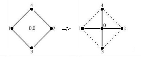
The shape on the right side is known in Finite Difference circles as a five point star.
It will be demonstrated here that it is possible to treat this Finite Difference pencil as if
it were a Finite Element. Let the coordinates of the parent five point star be given by:
$$
(0) = (0,0) \quad ; \quad \begin{cases} (1) = (-1,0) \quad ; \quad (2) = (+1,0) \\
(3) = (0,-1) \quad ; \quad (4) = (0,+1)\end{cases}
$$
Let function behaviour "inside" the five point star be approximated by a quadratic interpolation
between the function values at the vertices or nodal points, let $T$ be such a function and use
its Taylor expansion around the origin $(0)$:
$$
T(\xi,\eta) = T(0) + \frac{\partial T}{\partial \xi}(0).\xi
+ \frac{\partial T}{\partial \eta}(0).\eta
+ \frac{1}{2} \frac{\partial^2 T}{\partial \xi^2}(0).\xi^2
+ \frac{1}{2} \frac{\partial^2 T}{\partial \eta^2}(0).\eta^2
$$
Specify $T$ for the vertices with the basic polynomials of the five point star:
$$
T_0 = T(0)\\
T_1 = T(0) - \frac{\partial T}{\partial \xi}(0) + \frac{1}{2} \frac{\partial^2 T}{\partial \xi^2}(0)\\
T_2 = T(0) + \frac{\partial T}{\partial \xi}(0) + \frac{1}{2} \frac{\partial^2 T}{\partial \xi^2}(0)\\
T_3 = T(0) - \frac{\partial T}{\partial \eta}(0) + \frac{1}{2} \frac{\partial^2 T}{\partial \eta^2}(0)\\
T_4 = T(0) + \frac{\partial T}{\partial \eta}(0) + \frac{1}{2} \frac{\partial^2 T}{\partial \eta^2}(0)\\
\quad \mbox{ F.E. } \leftarrow \mbox{ F.D. }
$$
Solving these equations is not much of a problem
and well-known Finite Difference schemes are recognized:
$$
T(0) = T_0 \\
\frac{\partial T}{\partial \xi}(0) = \frac{T_2-T_1}{2}\\
\frac{\partial T}{\partial \eta}(0) = \frac{T_4-T_3}{2} \\
\frac{\partial^2 T}{\partial \xi^2}(0) = T_1-2T_0+T_2 \\
\frac{\partial^2 T}{\partial \eta^2}(0) = T_3-2T_0+T_4 \\
\quad \mbox{ F.D. } \leftarrow \mbox{ F.E. }
$$
Finite Element shape functions may be constructed as follows:
$$
T = N_0.T_0 + N_1.T_1 + N_2.T_2 + N_3.T_3 + N_4.T_4 = \\
T_0 + \frac{T_2-T_1}{2}\xi + \frac{T_4-T_3}{2}\eta
+ \frac{T_1-2T_0+T_2}{2}\xi^2 + \frac{T_3-2T_0+T_4}{2}\eta^2 =\\
(1-\xi^2-\eta^2)T_0 + \frac{1}{2}(-\xi+\xi^2)T_1 + \frac{1}{2}(+\xi+\xi^2)T_2
+\frac{1}{2}(-\eta+\eta^2)T_3 + \frac{1}{2}(+\eta+\eta^2)T_4 \\ \Longrightarrow \quad
\begin{cases}
N_0 = 1-\xi^2-\eta^2 \\
N_1 = (-\xi+\xi^2)/2\\
N_2 = (+\xi+\xi^2)/2\\
N_3 = (-\eta+\eta^2)/2\\
N_4 = (+\eta+\eta^2)/2
\end{cases}
$$
It is assumed that the same parameters $(\xi,\eta)$ are employed for the function $T$
as well as for the (global Cartesian) coordinates $x$ and $y$. Herewith it is expressed that
we have, as with the linear triangle and the bilinear quadrilateral, an isoparametric
transformation:
$$
\begin{cases}
x = N_0.x_0 + N_1.x_1 + N_2.x_2 + N_3.x_3 + N_4.x_4 \\
y = N_0.y_0 + N_1.y_1 + N_2.y_2 + N_3.y_3 + N_4.y_4
\end{cases} \quad \Longleftrightarrow \\
\begin{cases}
x =& x_0 + (x_2-x_1)/2\cdot\xi + (x_4-x_3)/2\cdot\eta\\
&+ \left[(x_1+x_2)/2-x_0\right]\cdot\xi^2 + \left[(x_3+x_4)/2-x_0\right]\cdot\eta^2 \\
y =& y_0 + (y_2-y_1)/2\cdot\xi + (y_4-y_3)/2\cdot\eta\\
&+ \left[(y_1+y_2)/2-y_0\right]\cdot\xi^2 + \left[(y_3+y_4)/2-y_0\right]\cdot\eta^2
\end{cases}
$$
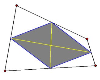
Now take a look at the picture below and let attention be shifted from the original quadrilateral
to the quadrilateral that joins the midpoints of the edges of the original. The latter is known as
the Varignon parallelogram
and it may be associated with our five point star.
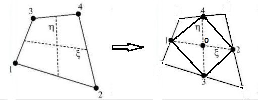
When doing so, the diagonals of the parallelogram become the local coordinate axes of the star and
by a well-known property of the diagonals of a parallelogram we have:
$$
\begin{cases} x_0 = (x_1+x_2)/2 \\ x_0 = (x_3+x_4)/2 \end{cases} \quad \mbox{and} \quad
\begin{cases} y_0 = (y_1+y_2)/2 \\ y_0 = (y_3+y_4)/2 \end{cases} \quad \Longrightarrow \\
\begin{cases}
x = x_0 + (x_2-x_1)/2.\xi + (x_4-x_3)/2.\eta \\
y = y_0 + (y_2-y_1)/2.\xi + (y_4-y_3)/2.\eta
\end{cases}
$$
Swithing back to the (numbering of) the original quadrilateral (on the left in the picture) we have:
$$\require{cancel}
\begin{array}{l}
x(\xi,\eta) = A_x + B_x.\xi + C_x.\eta\cancel{+ D_x.\xi.\eta} \\
y(\xi,\eta) = A_y + B_y.\xi + C_y.\eta\cancel{+ D_y.\xi.\eta}
\end{array} \qquad \mbox{ where: } \\
\begin{array}{ll}
A_x = \frac{1}{4} ( x_1 + x_2 + x_3 + x_4 ) & ; \quad
A_y = \frac{1}{4} ( y_1 + y_2 + y_3 + y_4 ) \\
B_x = \frac{1}{4} \left[(x_2 + x_4) - (x_1 + x_3)\right] & ; \quad
B_y = \frac{1}{4} \left[(y_2 + y_4) - (y_1 + y_3)\right] \\
C_x = \frac{1}{4} \left[(x_3 + x_4) - (x_1 + x_2)\right] & ; \quad
C_y = \frac{1}{4} \left[(y_3 + y_4) - (y_1 + y_2)\right] \\
\cancel{D_x = \frac{1}{4} ( + x_1 - x_2 - x_3 + x_4 )} & ; \quad
\cancel{D_y = \frac{1}{4} ( + y_1 - y_2 - y_3 + y_4 )}
\end{array}
$$
Which is precisely the original bilinear interpolation,
where the non-linear $\,\xi.\eta\,$ terms simply have been erased.
Due to the linearity achieved, the local parameters $(\xi,\eta)$ can easily be expressed now in the global coordinates $(x,y)$ :
$$
\begin{bmatrix} \xi \\ \eta \end{bmatrix} =
\begin{bmatrix} B_x & C_x \\ B_y & C_y \end{bmatrix}^{-1}
\begin{bmatrix} x-A_x \\ y-A_y \end{bmatrix}
$$
Because of the isoparametrics, exactly the same interpolation is applicable to any other
function $T$. Substitute $\,\xi(x,y),\eta(x,y)\,$ in:
$$
T(\xi,\eta) = A_T + B_T.\xi + C_T.\eta
\quad \mbox{ where: } \quad
\begin{cases}
A_T = \frac{1}{4} ( T_1 + T_2 + T_3 + T_4 ) \\
B_T = \frac{1}{4} \left[(T_2 + T_4) - (T_1 + T_3)\right] \\
C_T = \frac{1}{4} \left[(T_3 + T_4) - (T_1 + T_2)\right]
\end{cases}
$$
The idea is to evaluate function values at the midpoints of the edges of the bilinear quadrilateral.
Joining these midpoints together gives the Varignon parallelogram. Then employ the now linear interpolation of
this parallelogram as an extrapolation for points inside the original quadrilateral (under the assumption
that there is no problem with determining if a point is inside/outside an arbitrary convex quadrilateral
within an unstructured grid). Here is a visualization of the substitute interpolation. The original
quadrilateral is in black (with red vertices), the Varignon parallelogram is in blue, the $(\xi,\eta)$
coordinate axes are in yellow, the area covered by the substitute interpolation,
with $-1 < \xi+\eta < +1$ and $-1 < \xi-\eta < +1$ , is in grey. There are four
triangles remaining.
LATE EDIT. Continuing story at: