A point in the Euclidean plane is something without size. This means that we cannot really "see" a point.
Cast in analytical instead of geometrical terms: when seen "from above", a point at $(0,0)$ is a 2-D Dirac delta at the origin.
Likewise an (invisible) line $L(x,y)$ through the origin in the Euclidean plane is given by:
$$
L(x,y) = \delta(\cos(\phi).x+\sin(\phi).y)
$$
But virtually everybody who does geometry wants to make pictures, OK? What must be done then is "broaden" the Dirac delta.
We can consider instead a "fuzzyfied" point, smeared out over a small domain in the plane.
The fuzzyfication of that point can be modeled by a 2-D bell shaped function with a spread called $\sigma$ :
$$
P(x,y) = \frac{1}{2\pi\sigma^2}\: e^{-\frac{1}{2}\left[x^2+y^2\right]/\sigma^2}
$$
Likewise our line can be fuzzyfied ($\phi$ is the angle of the line's normal):
$$
L(x,y) = \frac{1}{\sigma\sqrt{2\pi}}\: e^{-\frac{1}{2}\left[\cos(\phi).x+\sin(\phi).y\right]^2/\sigma^2}
$$
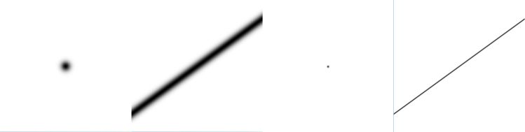
Then, all of a sudden, the point and the line become visible and can be drawn! In the picture below,
the viewport is $[-1,1]\times[-1,1]$ and the two spreads are $\sigma \in \{0.05,0.005\}$ respectively.
It should be emphasized that blurring of otherwise "sharp" points and lines is an important issue in Computer Graphics,
where the techniques for accomplishing this are called anti-aliasing. It should be noticed that the processing
of points and lines with finite sizes is mathematics too!
Anyway,
the function $P(x,y)$ can be sharpened to a point again. This is accomplished by a "limit" where the spread
becomes zero (assuming that it is legal in this forum to talk about such a limit):
$$
\delta(x,y) = \lim_{\sigma\rightarrow 0}
\frac{1}{2\pi\sigma^2}\:e^{-\frac{1}{2} \left[x^2+y^2\right]/\sigma^2}
$$
The same thing can be done for lines. Mind that the Gaussian does not belong to the test functions
with compact support. And yet it converges to the Dirac delta.
Now I don't know what mathematicians think about this, but as a physicist I find that the whole of (Euclidean) geometry,
when viewed in this way, is a bunch of Dirac deltas all over the place. They have been there all the time, in disguise.
Physicists didn't invent them. Expecially the treatment of lines should be memorized when reading what follows.
I will try to show how useful it is.
The problem that will be considered is the
"Inside/Outside problem". I'm only talking about the planar (2-D) case here: just think of a boundary enclosing a certain domain
of interest. Then, as a human, one can decide almost immediately whether a point is inside or outside this domain:
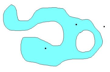
Now try to share that experience with a computer! And I bet we'll be on speaking terms quite soon.
In cartesian coordinates
The above becomes somewhat less trivial as soon as (the fuzzyfication of) a
point is integrated over a certain area, which is enclosed by some curve:
$$
\iint\frac{1}{2\pi\sigma^2}\:e^{-\frac{1}{2} \left[x^2+y^2\right]/\sigma^2} \: dx\,dy
$$ $$
= \iint
\frac{1}{\sigma\sqrt{2\pi}} e^{-\frac{1}{2} x^2/\sigma^2}
\frac{1}{\sigma\sqrt{2\pi}} e^{-\frac{1}{2} y^2/\sigma^2} \: dx\,dy
$$
According to Green's Theorem ,
any such area integral may be converted into a contour integral. As follows:
$$
\iint \left( \frac{\partial Q}{\partial x} - \frac{\partial P}{\partial y} \right)
\, dx \, dy = \oint \left( P\,dx + Q\,dy \right)
$$
Where the line integral must be evaluated along the contour enclosing the area
of interest.
We opt for the following. Let the function $P(x,y)$ be zero everywhere and let
the function $Q(x,y)$ be defined by:
$$
Q(x,y) = \operatorname{erf}\left(\frac{x}{\sigma}\right) \;
\frac{1}{\sigma\sqrt{2\pi}} e^{-\frac{1}{2} y^2/\sigma^2} \quad \Longrightarrow
\\ \frac{\partial Q}{\partial x} = \frac{1}{\sigma\sqrt{2\pi}} e^{-\frac{1}{2} x^2/\sigma^2}
\frac{1}{\sigma\sqrt{2\pi}} e^{-\frac{1}{2} y^2/\sigma^2}
$$
Which is exactly what we want. Now the result of Green's Theorem becomes:
$$
\iint \frac{\partial Q}{\partial x} \,dx\,dy = \oint Q\,dy = \oint \operatorname{erf}
\left(\frac{x}{\sigma}\right) \frac{1}{\sigma\sqrt{2\pi}} e^{-\frac{1}{2} y^2/\sigma^2} \,dy
$$
In the limiting case, when $\sigma \rightarrow 0$ , the exponential function
becomes a Dirac delta and the $\operatorname{erf}$ function becomes an integrated Dirac delta, which is the Heaviside function:
$$
H(x) = \begin{cases} 0 & \mbox{for} & x < 0 \\ 1 & \mbox{for} & x > 0 \end{cases}
$$
Thus we find:
$$
\lim_{\sigma\rightarrow 0} \oint \operatorname{erf}\left(\frac{x}{\sigma}\right)
\frac{1}{\sigma\sqrt{2\pi}} e^{-\frac{1}{2} y^2/\sigma^2} \,dy = \oint H(x) \, \delta(y) \, dy
$$
In polar coordinates
But there are other ways to look at the integral:
$$
\iint \frac{1}{2\pi\sigma^2}\:e^{-\frac{1}{2} \left[x^2+y^2\right]/\sigma^2} \: dx\,dy
$$
For example, replace the Cartesian $(x,y)$ system by polar coordinates $(r,\phi)$ :
$$
\iint \frac{1}{2\pi\sigma^2}\: e^{-\frac{1}{2} \left[x^2+y^2\right]/\sigma^2} \: dx\,dy
= \iint \frac{1}{2\pi\sigma^2}\: e^{-\frac{1}{2} r^2/\sigma^2} \: r\,dr\,d\phi
$$
The latter integral can be evaluated as follows:
$$
\iint \frac{1}{2\pi\sigma^2}\: e^{-\frac{1}{2} r^2/\sigma^2} \: r\,dr\,d\phi =
\frac{1}{2\pi} \int_{\phi} \left[ - \int_r e^{-\frac{1}{2} (r/\sigma)^2}
d\left\{-\frac{1}{2} (r/\sigma)^2\right\} \right] d\phi
$$
If we take the limit for $\sigma \rightarrow 0$ of the integral between square
brackets, then it is reduced to unity:
$$
\lim_{\sigma \rightarrow 0} - \int_0^{-\frac{1}{2} R^2/\sigma^2} e^t \, dt =
\lim_{\sigma \rightarrow 0} \left[ 1 - e^{-\frac{1}{2} (R/\sigma)^2} \right] = 1
$$
Here $R$ denotes the distance of the boundary curve to the origin. If it may be
assumed that the origin is distinct from the boundary, then for $\sigma
\rightarrow 0$ the quotient $R/\sigma$ approaches infinity and the exponential
function becomes zero indeed. So we are left with:
$$
\iint \frac{1}{2\pi\sigma^2}\: e^{-\frac{1}{2} r^2/\sigma^2}
\: r\,dr\,d\phi \;\to\; \frac{1}{2\pi} \oint d\phi
$$
Combining the cartiesian coordinates with the polar coordinates result leads to the
following, which might be a hitherto unknown
Theorem
$$
\boxed{\large \oint H(x) \, \delta(y) \, dy = \frac{1}{2\pi} \oint d\phi } \\
\mbox{Crossing number = Winding number}
$$
Here is a visualization:
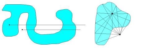
Left hand side of formula and picture.
Draw a horizontal line $\,= \delta(y)\,$ from the point of interest to the right,
towards infinity (which is as far as necessary). A line to the left would have no sense,
because the Heaviside function $H(x)$ is zero there, so there cannot be a
sensible contribution. (This should be recognized as a clipping problem)
The delta function is integrated in vertical direction over all places where
our line to the right intersects the boundary. This results in a contribution
$+1$ where $dy > 0$ (upwards) or $-1$ where $dy < 0$ (downwards). For the inside
point (blue area) summing up all the $\pm 1$ contributions will result in $1$ .
For the outside point (white area) summing up all these contributions
will result in $0$ . This "ray shooting" method is actually a classic.
However, most treatments of it barely scratch the surface. It's very important
to distinguish all special cases carefully. Such as the nine possible positions
of a(n infinitesimal) contour line segment $(p,q)$ with respect to the ray:
                      q      p  p-q
 >         q          |   p  |
 = -----q--|--p--p-q--p---|--q-----
 <      |  p  |           q
   p-q  p     q
    0   1  2  3   4   5   6  7   8
Right hand side of formula and picture.
This is recognized as the winding number. Algorithmically speaking,
using the winding number is not as efficient, because angles are expensive to calculate.
For the inside point (blue area) summing up the angles, while traversing the boundary
in counter-clockwise direction, results in $2\pi$ . Therefore the outcome of the winding
number integral is $1$ . For the outside point (white area) summing up the angles, while
traversing the boundary in counter-clockwise direction, results in $0$ . Therefore the
outcome of the winding number integral is $0$ .
Apart from the (barely proven ?) properties mentioned by the OP, another property pops up in the above.
In the proof of our Theorem, use has been made of a property that is typical for exponential functions,
and it is crucial for our argument:
$$
e^{x^2}e^{y^2} = e^{x^2+y^2} = e^{r^2}
$$
But I can't remember that there is a similar property in the standard list (if there is one) for Dirac deltas.
The property is only there if the Dirac deltas in place are "limits" of Gaussians. Correct me if I'm wrong.
This might suggest that perhaps there is no such comprehensive list at all and that it all depends upon the
choice of the functions that are converging to the Dirac delta in place. The good news is that, at least with
Gaussian distributions as the test functions, the Dirac delta can easily be generalized to multiple dimensions $n$:
$$
\delta(x_1,x_2,\cdots,x_n) = \lim_{\sigma\to 0}\frac{e^{(x_1^2+x_2^2+\cdots+x_n^2)/2\sigma^2}}{\left(2\pi\sigma^2\right)^{n/2}}
$$