Now forget about the moments for a moment :-)
With a Least Squares Method, on the other hand, the following integral is minimized:
$$
\int_0^1 \left[ f(x)-p(x) \right]^2 dx = \int_0^1 \left[ f(x)-\sum_{k=0}^{n-1} a_k x^k \right]^2 dx =
\mbox{minimum}(a_0,a_1,a_2,\cdots,a_{n-1})
$$
Take partial derivatives $\partial/\partial a_k \; ; \; k=0,1,2,\cdots,n-1$ to find the minimum:
$$
\int_0^1 x^k \left[ f(x) - \sum_{j=0}^{n-1} a_j x^j \right] dx = 0 \quad \Longleftrightarrow \quad
\sum_{j=0}^{n-1} \frac{1}{k+j+1} a_j = M_k
$$
Which turns out to be exactly the same system of linear (and ill-conditioned) equations as above.
Thus we conclude that finding a polynomial with the same first $n$ moments of a given function
is equivalent with finding the least squares best fit polynomial of order $(n-1)$ to that function,
WLOG at the interval $\left[0,1\right]$ . Now take the limit for $n\rightarrow\infty$ and we're done, it seems.
So, any real valued function defined at a finite interval can be resolved (in a least squares sense)
from its sequence of moments and there are no restrictions on these moments.
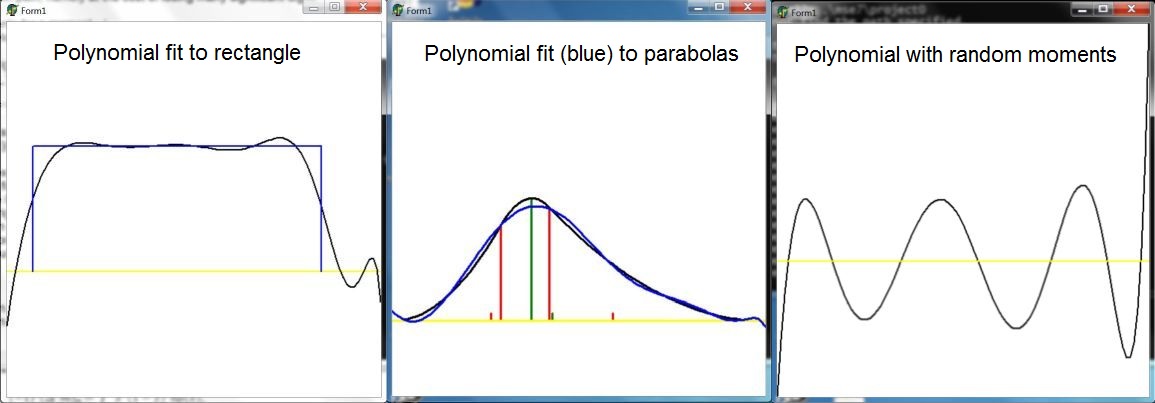
It is noted that the functions found are, in general, no probability distributions and can be quite "wild".
At last, there is a residual (i.e. error estimate) to take into account: $$ \int_0^1 \left[ f(x)-p(x) \right]^2 dx = \int_0^1 f(x)^2 dx - 2 \sum_{k=0}^{n-1} a_k \int_0^1 f(x) x^k dx + \sum_{k=0}^{n-1} a_k \sum_{j=0}^{n-1} a_j \int_0^1 x^k x^j dx = \\ = \int_0^1 f(x)^2 dx - \sum_{k=0}^{n-1} a_k M_k $$ It is worrysome that, sometimes but too often, the residual turns out to be negative (numerically). How can that happen? I think it means that our numerical calculations just aren't much reliable, due to poor condtioning of the Hilbert matrix.
With histogram functions, there is NO equivalent between the Moment problem and Least Squares:
$$
\int_0^1 \left[ f(x) - h(x) \right]^2 dx = \sum_{k=0}^{n-1} \int_{k/n}^{(k+1)/n}
\left[ f(x) - f_k \right]^2 dx = \mbox{minimum}(f_0,f_1,f_2,\cdots,f_{n-1})
$$
Take partial derivatives $\partial/\partial f_k \; ; \; k=0,1,2,\cdots,n-1$ to find the minimum:
$$
\int_{k/n}^{(k+1)/n} \left[ f(x) - f_k \right] dx = 0 \quad \Longleftrightarrow \quad
\frac{\int_{k/n}^{(k+1)/n} f(x)\, dx}{(k+1)/n-k/n} = f_k
$$
Meaning that any $f_k$ is the mean of the function $f(x)$ over the interval $\left[k/n,(k+1)/n\right]$ .
At last, there is a residual (i.e. error estimate) to take into account:
$$
\int_0^1 \left[ f(x)-h(x) \right]^2 dx = \int_0^1 f(x)^2 dx - \sum_{k=0}^{n-1} \left[\frac{k+1}{n}-\frac{k}{n}\right] f_k^2
$$
Numerical calculations with Histogram Moments reveal that the results seem to be approximately what
one would expect with Least Squares (see: Histogram fit to parabolas). But it is not at all obvious
(to me at least) that the two methods converge to the same thing.
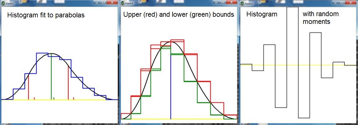
It is also possible to have histograms as $\color{red}{upper}$ and $\color{green}{lower}$ bounds to a function. Then the (raw) moments of the function are in between the (raw) moments of the histograms. Given an infinite precision computer that does not suffer from ill conditioned equations, then for $n\to\infty$ this fact would prove that an infinite sequence of moments determines the function. It is shown in the picture, though, that solving the histogram equations gives $\color{red}{upper}$ and $\color{green}{lower}$ histograms that are seen to be different from the exact ones, thus confirming again the dreadful conditioning with even moderate size (< $10$) of the equations system. References:

The most trivial histogram function $y = f(x)$ at the interval $\left[0,1\right]$ may be defined as follows:
$$
y = f_0 \quad \mbox{for} \quad 0 < x < 1
$$
The zero'th moment of this function is: $m_0 = f_0$ and the function as a whole is trivially
determined by its zero'th moment: $f_0 = m_0$ .
A bit less trivial histogram function $y = f(x)$ at the same interval may be defined as follows:
$$
y = f_0 \quad \mbox{for} \quad 0 < x < \frac{1}{2} \quad ;
\quad y = f_1 \quad \mbox{for} \quad \frac{1}{2} < x < 1
$$
The first two moments of this function are:
$$
\left[ \begin{array}{c} m_0 \\ m_1 \end{array} \right] =
\left[ \begin{array}{cc} 1/2 & 1/2 \\ 1/8 & 3/8 \end{array} \right]
\left[ \begin{array}{c} f_0 \\ f_1 \end{array} \right]
$$
With the inverse matrix it yields:
$$
\left[ \begin{array}{c} f_0 \\ f_1 \end{array} \right] =
\left[ \begin{array}{cc} 3 & -4 \\ -1 & 4 \end{array} \right]
\left[ \begin{array}{c} m_0 \\ m_1 \end{array} \right]
$$
Thus the function as a whole is determined by $m_0$ and $m_1$ . If there are no restrictions
upon the function values, then there are no restrictions upon the moments.
If we demand, though, that the function values are positive, then further restrictions are
imposed upon the moments. Assume that $m_0 > 0$ and define the mean $\mu = m_1/m_0$ :
$$
\left. \begin{array}{l} \frac{3}{4} - \frac{m_1}{m_0} > 0 \\
-\frac{1}{4} + \frac{m_1}{m_0} > 0 \end{array}\right\} \quad \Longrightarrow
\quad \frac{1}{4} < \mu < \frac{3}{4}
$$
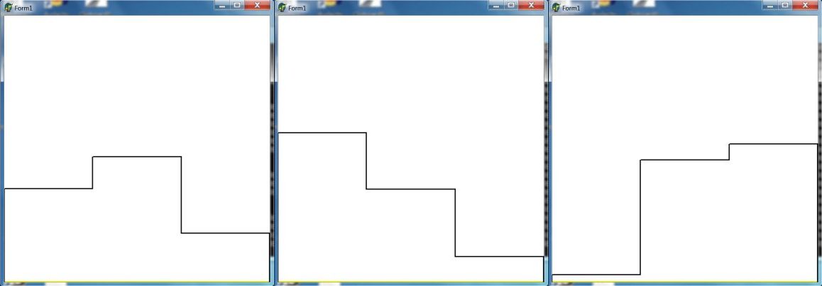
Another sample histogram function $y = f(x)$ at the same interval may be defined as follows:
$$
y = f_k \quad \mbox{for} \quad \frac{k}{3} < x < \frac{k+1}{3} \quad : \quad k = 0,1,2
$$
The first three moments are:
$$
\left[ \begin{array}{c} m_0 \\ m_1 \\ m_2 \end{array} \right] =
\left[ \begin{array}{ccc} 1/3 & 1/3 & 1/3 \\ 1/18 & 1/6 & 5/18 \\ 1/81 & 7/81 & 19/81 \end{array} \right]
\left[ \begin{array}{c} f_0 \\ f_1 \\ f_2 \end{array} \right]
$$
Calculating the inverse matrix yields:
$$
\left[ \begin{array}{c} f_0 \\ f_1 \\ f_2 \end{array} \right] =
\left[ \begin{array}{ccc} 11/2 & -18 & 27/2 \\ -7/2 & 27 & -27 \\ 1 & -9 & 27/2 \end{array} \right]
\left[ \begin{array}{c} m_0 \\ m_1 \\ m_2 \end{array} \right]
$$
Thus the function as a whole is determined by $m_0,m_1,m_2$ . If there are no restrictions
upon the function values, then there are no restrictions upon the moments.
If we demand, though, that the function values are positive, then further restrictions are
imposed upon the moments. Assume again that $m_0 > 0$ and define $x = m_1/m_0$ and $y = m_2/m_0$
for the sake of displaying results in a diagram (at the bottom of this answer). Then:
$$
\left. \begin{array}{l} f_0 > 0 \\ f_1 > 0 \\ f_2 > 0 \end{array} \right\}
\quad \Longleftrightarrow \quad \left\{ \begin{array}{l}
y - 4/3 x + 11/27 > 0 \\
y - x + 7/54 < 0 \\
y - 2/3 x + 2/27 < 0 \end{array} \right.
$$
Three straight lines delineate the $\color{blue}{blue}$ area of an obtuse triangle
with vertices $(1/6,1/27) , (5/6,19/27) , (1/2,7/27)$ , as shown in the diagram at the bottom.
The moments must be such that $(x,y)$ values are within this triangle;
it has
an area of $1/27$ .
A further restriction upon the histogram might be that it is sort of a concave function.
To be more precise, this would mean that the second order derivative is negative, which is
of course impossible with histograms. A reasonable substitute is that the well known
discretization of the second order derivative should be negative:
$$
f_0 - 2 f_1 + f_2 < 0 \quad \Longleftrightarrow \quad y - x + 1/6 < 0
$$
While the equations for $f_0 > 0$ and $f_2 > 0$ remain the same.
Three straight lines delineate the $\color{green}{green}$ area of an obtuse triangle
with vertices $(5/18,1/9) , (13/18,5/9) , (1/2,7/27)$ , as shown in the diagram at the bottom.
The moments must be such that $(x,y)$ values are within this triangle;
it has
an area of $4/243 < 1/27$ .
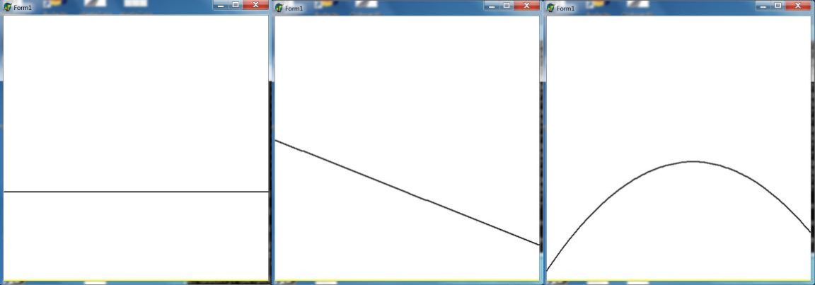
The most trivial polynomial function $y = p(x)$ at the interval $\left[0,1\right]$ is: $y = a_0$
with a zero'th order moment $= m_0$ . This case is identical to the trivial histogram above.
A somewhat less trivial polynomial $y = p(x)$ at the same interval is the linear one: $y = a_0 + a_1 x$ .
Its first two moments are:
$$
\left[ \begin{array}{c} m_0 \\ m_1 \end{array} \right] =
\left[ \begin{array}{cc} 1 & 1/2 \\ 1/2 & 1/3 \end{array} \right]
\left[ \begin{array}{c} a_0 \\ a_1 \end{array} \right]
$$
With the inverse (symmetric & integer) matrix it yields:
$$
\left[ \begin{array}{c} a_0 \\ a_1 \end{array} \right] =
\left[ \begin{array}{cc} 4 & -6 \\ -6 & 12 \end{array} \right]
\left[ \begin{array}{c} m_0 \\ m_1 \end{array} \right]
$$
Thus the function as a whole is determined by $m_0$ and $m_1$ . If there are no restrictions
upon the function values, then there are no restrictions upon the moments.
If we demand, though, that the function values are positive, then further restrictions are
imposed upon the moments. Assume that $m_0 > 0$ and define the mean $\mu = m_1/m_0$ :
$$
\left. \begin{array}{l} \frac{2}{3} - \frac{m_1}{m_0} > 0 \\
-\frac{1}{3} + \frac{m_1}{m_0} > 0 \end{array}\right\} \quad \Longrightarrow
\quad \frac{1}{3} < \mu < \frac{2}{3}
$$
Another sample polynomial $y = p(x)$ at the same interval may be defined as follows:
$$
y = a_0 + a_1 x + a_2 x^2
$$
It's a parabola, of course. The first three moments are:
$$
\left[ \begin{array}{c} m_0 \\ m_1 \\ m_2 \end{array} \right] =
\left[ \begin{array}{ccc} 1 & 1/2 & 1/3 \\ 1/2 & 1/3 & 1/4 \\ 1/3 & 1/4 & 1/5 \end{array} \right]
\left[ \begin{array}{c} a_0 \\ a_1 \\ a_2 \end{array} \right]
$$
Calculating the (symmetric & integer) inverse matrix yields:
$$
\left[ \begin{array}{c} a_0 \\ a_1 \\ a_2 \end{array} \right] =
\left[ \begin{array}{ccc} 9 & -36 & 30 \\ -36 & 192 & -180 \\ 30 & -180 & 180 \end{array} \right]
\left[ \begin{array}{c} m_0 \\ m_1 \\ m_2 \end{array} \right]
$$
Thus the function as a whole is determined by $m_0,m_1,m_2$ . If there are no restrictions
upon the function values, then there are no restrictions upon the moments.
If we demand, though, that function values are positive, then further restrictions are
imposed upon the moments. Assume again that $m_0 > 0$ and define $x = m_1/m_0$ and $y = m_2/m_0$
for the sake of being able to display results in a diagram.
Then assume that $p(0) > 0$ , $p(1) > 0$ and that the parabola is concave (i.e. has a maximum).
So what we have again is a function that is positive and concave:
$$
\left. \begin{array}{l} a_0 > 0 \\ a_0+a_1+a_2 > 0 \\ a_2 < 0 \end{array} \right\}
\quad \Longleftrightarrow \quad \left\{ \begin{array}{l}
y - 6/5 x + 3/10 > 0 \\
y - 4/5 x + 1/10 > 0 \\
y - x + 1/6 < 0 \end{array} \right.
$$
Three straight lines delineate the $\color{red}{red}$ area of an obtuse triangle
with vertices $(1/3,1/6) , (2/3,1/2) , (1/2,3/10)$ , as shown in the diagram below.
The moments must be such that $(x,y)$ values are within this triangle;
the triangle
has an an area of $1/180 < 4/243 < 1/27$ .
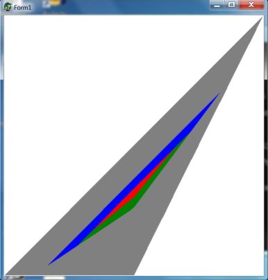
The grey area comes from restrictions on moments as explained in a Wikipedia
reference .
The moment sequence $\; m_0,m_1,m_2, \cdots , m_n , \cdots \;$ is completely monotonic iff:
$$
(-1)^k(\Delta^k m)_n \ge 0 \quad \mbox{for all} \quad n,k \ge 0
\qquad \mbox{with} \qquad (\Delta m)_n = m_{n+1} - m_n
$$
In order to avoid trivialities, strict inequalitites will be assumed.
Let's do it, but only for $m_0,m_1,m_2$ :
$$
n=0 \; , \; k=0 \quad : \qquad m_0 > 0 \\
n=1 \; , \; k=0 \quad : \qquad m_1 > 0 \\
n=2 \; , \; k=0 \quad : \qquad m_2 > 0 \\
n=0 \; , \; k=1 \quad : \qquad - (m_1 - m_0) > 0 \\
n=1 \; , \; k=1 \quad : \qquad - (m_2 - m_1) > 0 \\
n=0 \; , \; k=2 \quad : \qquad (\Delta m)_1 - (\Delta m)_0
= m_2 - 2 m_1 + m_0 > 0
$$
Summarizing and putting $\;x = m_1/m_0\;$ and $\;y = m_2/m_0\;$ for visualization purposes:
$$
y > 0 \quad ; \quad y < x \quad ; \quad y > 2 x - 1
$$
Three straight lines delineate the $\color{gray}{grey}$ area of an obtuse triangle
with vertices $(0,0) , (1/2,0) , (1,1)$ as shown in the above diagram. The triangle has an an area of $1/4$ .
By coincidence,
the $\color{red}{red}$ polynomial triangle is a proper subset of the $\color{green}{green}$
histogram triangle is a proper subset of the $\color{blue}{blue}$ histogram triangle
(is a proper subset of the $\color{grey}{grey}$ "Hausdorff" triangle).
But the question is: does there exist something like "coincidence" in mathematics?