The formula $\;\oint H(x) \, \delta(y) \, dy = \frac{1}{2\pi} \oint d\phi\;$
Explanation - everything real-valued:
$$
(x,y) = \mbox{cartesian coordinates} \\
\phi = \mbox{angle, in polar coordinates} \\
H(x) = \begin{cases} 0 & \mbox{for} & x < 0 \\ 1 & \mbox{for} & x > 0 \end{cases} \quad \mbox{: Heaviside function}\\
\delta(y) = \begin{cases} 0 & \mbox{for} & y \ne 0 \\ \infty & \mbox{for} & y = 0 \end{cases} \quad \mbox{and} \quad
\int_{-\infty}^{+\infty} \delta(y) \,dy = 1 \quad \mbox{: Dirac delta}
$$
The meaning of the formula is a topological one:
Crossing number = Winding number
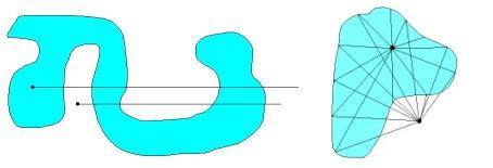
Here is a visualization. WLOG the origin $(0,0)$ is taken at the black dots inside/outside a domain.
The integrations are carried out over the boundary of that domain.
A point in the plane is something without size. We can consider instead a fuzzyfied point, smeared out
over a small domain in the plane. Cast in more mathematical terms: a point at $(0,0)$ is a Dirac delta
at the origin. The fuzzyfication of that point can be modelled by a 2-D bell shaped function with a
spread called $\sigma$ :
$$
G(x,y) = \frac{1}{2\pi\sigma^2}\: e^{-\frac{1}{2}\left[x^2+y^2\right]/\sigma^2}
$$
The function $G(x,y)$ can be sharpened to a point. This is accomplished by a limit where the spread
becomes zero:
$$
\lim_{\sigma\rightarrow 0}
\frac{1}{2\pi\sigma^2}\:e^{-\frac{1}{2} \left[x^2+y^2\right]/\sigma^2}
$$
Cartesian coordinates
The above becomes somewhat less trivial as soon as (the fuzzyfication of) a
point is integrated over a certain area, which is enclosed by some curve:
$$
\iint\frac{1}{2\pi\sigma^2}\:e^{-\frac{1}{2} \left[x^2+y^2\right]/\sigma^2} \: dx\,dy
$$ $$
= \iint
\frac{1}{\sigma\sqrt{2\pi}} e^{-\frac{1}{2} x^2/\sigma^2}
\frac{1}{\sigma\sqrt{2\pi}} e^{-\frac{1}{2} y^2/\sigma^2} \: dx\,dy
$$
According to Green's Theorem ,
any such area integral may be converted into a contour integral. As follows:
$$
\iint \left( \frac{\partial Q}{\partial x} - \frac{\partial P}{\partial y} \right)
\, dx \, dy = \oint \left( P\,dx + Q\,dy \right)
$$
Where the line integral must be evaluated along the contour enclosing the area
of interest. Converting a line integral into an area integral is easy. But the
reverse, converting an area integral into a line integral, requires some more
ingenuity. In our case, though, there exists more than one possibility to do it.
We opt for the following. Let the function $P(x,y)$ be zero everywhere and let
the function $Q(x,y)$ be defined by:
$$
Q(x,y) = \operatorname{erf}\left(\frac{x}{\sigma}\right) \;
\frac{1}{\sigma\sqrt{2\pi}} e^{-\frac{1}{2} y^2/\sigma^2} \quad \Longrightarrow
\\ \frac{\partial Q}{\partial x} = \frac{1}{\sigma\sqrt{2\pi}} e^{-\frac{1}{2} x^2/\sigma^2}
\frac{1}{\sigma\sqrt{2\pi}} e^{-\frac{1}{2} y^2/\sigma^2}
$$
Which is exactly what we want. Now the result of Green's Theorem becomes:
$$
\iint \frac{\partial Q}{\partial x} \,dx\,dy = \oint Q\,dy = \oint \operatorname{erf}
\left(\frac{x}{\sigma}\right) \frac{1}{\sigma\sqrt{2\pi}} e^{-\frac{1}{2} y^2/\sigma^2} \,dy
$$
In the limiting case, when $\sigma \rightarrow 0$ , the exponential function
becomes a Dirac delta and the $\operatorname{erf}$ function becomes an integrated Driac delta,
which is the Heaviside function. Thus we find:
$$
\lim_{\sigma\rightarrow 0} \oint \operatorname{erf}\left(\frac{x}{\sigma}\right)
\frac{1}{\sigma\sqrt{2\pi}} e^{-\frac{1}{2} y^2/\sigma^2} \,dy = \oint H(x) \, \delta(y) \, dy
$$
Polar coordinates
But there are a myriad other ways to look at the integral:
$$
\iint \frac{1}{2\pi\sigma^2}\:e^{-\frac{1}{2} \left[x^2+y^2\right]/\sigma^2} \: dx\,dy
$$
For example, replace the Cartesian $(x,y)$ system by polar coordinates $(r,\phi)$ :
$$
\iint \frac{1}{2\pi\sigma^2}\: e^{-\frac{1}{2} \left[x^2+y^2\right]/\sigma^2} \: dx\,dy
= \iint \frac{1}{2\pi\sigma^2}\: e^{-\frac{1}{2} r^2/\sigma^2} \: r\,dr\,d\phi
$$
The latter integral can be evaluated as follows:
$$
\iint \frac{1}{2\pi\sigma^2}\: e^{-\frac{1}{2} r^2/\sigma^2} \: r\,dr\,d\phi =
\frac{1}{2\pi} \int_{\phi} \left[ - \int_r e^{-\frac{1}{2} (r/\sigma)^2}
d\left\{-\frac{1}{2} (r/\sigma)^2\right\} \right] d\phi
$$
If we take the limit for $\sigma \rightarrow 0$ of the integral between square
brackets, then it is reduced to unity:
$$
\lim_{\sigma \rightarrow 0} - \int_0^{-\frac{1}{2} R^2/\sigma^2} e^t \, dt =
\lim_{\sigma \rightarrow 0} \left[ 1 - e^{-\frac{1}{2} (R/\sigma)^2} \right] = 1
$$
Here $R$ denotes the distance of the boundary curve to the origin. If it may be
assumed that the origin is distinct from the boundary, then for $\sigma
\rightarrow 0$ the quotient $R/\sigma$ approaches infinity and the exponential
function becomes zero indeed. So we are left with:
$$
\iint \frac{1}{2\pi\sigma^2}\: e^{-\frac{1}{2} r^2/\sigma^2}
\: r\,dr\,d\phi = \frac{1}{2\pi} \oint d\phi
$$
Combining the cartiesian coordinates with the polar coordinates result leads to the following
Main Theorem
$$
\boxed{\large \oint H(x) \, \delta(y) \, dy = \frac{1}{2\pi} \oint d\phi } \\
\mbox{Crossing number = Winding number}
$$
Draw a horizontal line from the point of interest to the right, towards
infinity (which is as far as necessary). A line to the left would have no sense,
because the Heaviside function $H(x)$ is zero there, so there cannot be a
sensible contribution. (This should be recognized as a clipping problem.)
The delta function is integrated in vertical direction over all places where
our line to the right intersects the boundary. This results in a contribution
$+1$ where $dy > 0$ (upwards) or $-1$ where $dy < 0$ (downwards). For the inside
point (blue area) summing up all the $\pm 1$ contributions will result in $1$ .
For the outside point (white area) summing up all these contributions
will result in $0$ . This "ray shooting" method is actually a classic.
However, most treatments of it barely scratch the surface. It's very important
to distinguish all special cases carefully. Such as the $9$ possible positions
of a contour line segments $(p,q)$ with respect to the ray:
                      q      p  p-q
 >         q          |   p  |
 = -----q--|--p--p-q--p---|--q-----
 <      |  p  |           q
   p-q  p     q
    0   1  2  3   4   5   6  7   8
The right hand side is recognized as the winding number. Algorithmically speaking,
using the winding number is not as efficient, because angles are expensive to calculate.
For the inside point (blue area) summing up the angles, while traversing the boundary
in counter-clockwise direction, results in $2\pi$ . Thus the outcome of the winding number integral is $1$ .
For the outside point (white area) summing up the angles, while traversing the boundary
in counter-clockwise direction, results in $0$ . Thus the outcome of the winding number integral is $0$ .