previous overview next
Product Function
$
\def \half {\frac{1}{2}}
\def \kwart {\frac{1}{4}}
\def \EN {\quad \mbox{and} \quad}
\def \OF {\quad \mbox{or} \quad}
\def \hieruit {\quad \Longrightarrow \quad}
\def \slechts {\quad \Longleftrightarrow \quad}
$
The product of the off-diagonal coefficients at the coarsened grid can be
expressed as a function of the product of the off-diagonal terms at the refined
grid:
$$
a'.b' = \frac{a^2}{1 - 2.a.b} \; \frac{b^2}{1 - 2.a.b}
= \left(\frac{a.b}{1 - 2.a.b}\right)^2
$$ Or: $$
y = \left(\frac{x}{1 - 2.x}\right)^2 \qquad \mbox{where} \qquad
y = a'.b' \EN x = a.b
$$
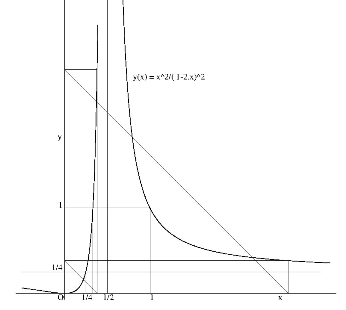
At first, we make a sketch of the function which relates the product $a'.b'$ on
the finer grid to the product $a.b$ on the coarser grid.
That is, the function $y = x^2/(1-2.x)^2$ .
The function has two asymptotes, a vertical one for $x = 1/2$ (denominator = 0)
and a horizontal one for $y = 1/4$:
$$
\lim_{x \rightarrow \pm \infty} \left( \frac{x}{1 - 2.x} \right)^2 =
\lim_{x \rightarrow \pm \infty} \left( \frac{1}{2 - 1/x} \right)^2 =
\frac{1}{4}
$$
We want to make a small step aside now, and ask attention for a subject which
is on the experimental side and therefore a bit different from the mainstream
theoretical argument.
While having a look at the graphics, the reader may wonder how these pictures
were created. The answer is that most of the figures were composed by making
use of native PostScript. This seems to be weird at first sight, but it
should be remarked here that PostScript is, in fact, a full blown programming
language. (Moreover, it is a language which offers no special difficulties to
someone who has been an experienced FORTH programmer.) Much of the
theory in this document has been accompanied by numerical experiments. These
experiments were implemented and carried out a great deal in (Turbo) Pascal.
But, since PostScript is a programming language, nothing has prevented us from
having carried out some of these numerical experiments entirely in PostScript.
That's why the source code of the pictures in this document actually contain
more information than may be displayed. It is suggested herewith that the PSF
(PostScriptFile) programs, as delivered with this document, may be interesting
as such. Having said this, let's return to theory, starting with the figure
below. Click On Pic for viewing the PostScript code:
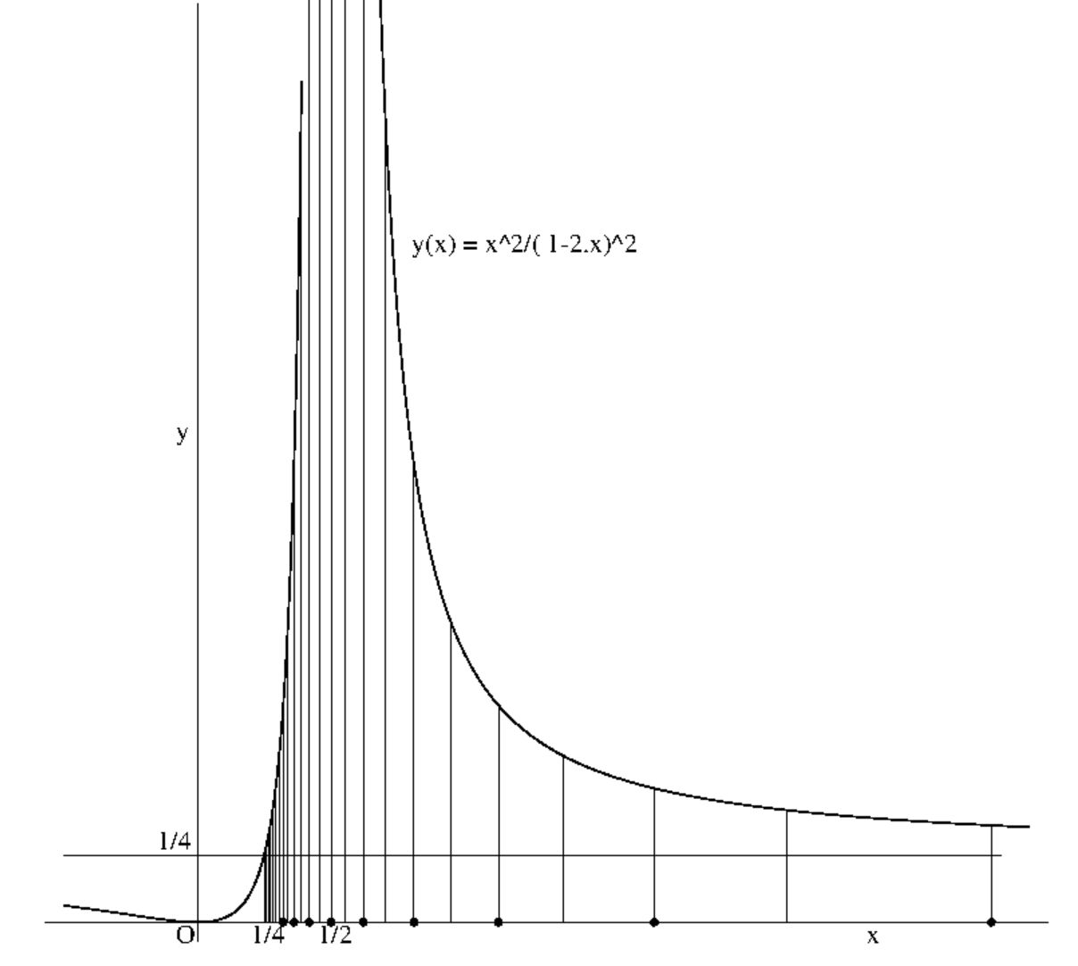
With grid coarsening, the function is used iteratively. Get started with
a certain value of $x$ and the accompanying value of $y$ can be calculated. But
this value of $y$ serves as the next $x$ value for the function $y$, as soon as
the grid is coarsened again. In general, we obtain an assembly of the form:
$$
y\left(y\left(y\left(y\left(y ... y(x)\right)\right)\right)\right)
$$
It may be questioned if there exist values of $x$ which are are such that,
after coarsening of the grid, the same value $x = y(x)$ is acquired again.
Such values will remain the same during all stages of the grid coarsening
process. For this reason, such values of $x$ are called stationary or
invariant points of the function. They are found as follows:
$$
x = \left( \frac{x}{2.x-1} \right)^2 \hieruit x = 0 \OF
1.(2.x-1)^2 = x \hieruit $$ $$ x^2 - \frac{5}{4} x + 1
= (x - 1)(x - \frac{1}{4}) = 0
$$
Herewith invariant points are found to be:
$$
x = 0 \OF x = 1 \OF x = \kwart
$$
The value $1/3$, being useful because of the condition $a.b < 1/3 < 1/2$, is
mapped on the stationary value $1$:
$$
\left( \frac{1/3}{1-2.1/3} \right)^2 = 1
$$
But the above list of invariant points is not exhaustive, another possibility
being that there exist two points instead of one. After having obtained
the point with label (1) in one iteration, the point with label (2) is reached
in the next iteration. Then the point with label (1) is obtained again, and so
on and so forth. We must solve an equation with $1/x$ instead of $x$:
$$
\frac{1}{x} = \left( \frac{x}{2.x-1} \right)^2 \hieruit (2.x-1)^2 = x^3
\hieruit x^3 - 4.x^2 + 4.x - 1 = 0
$$
An equation of the third degree. However, we already know that $x=1/x=1$ must
be a solution of it. Hence we can perform a division:
$$
\frac{ x^3 - 4.x^2 + 4.x - 1 }{ x - 1 } = x^2 - 3.x + 1 = 0
$$
The roots of the equation are herewith found to be:
$$
x_1 = 1 \OF x_2 = \frac{3}{2} + \frac{\sqrt{5}}{2} \approx 2.618
\OF x_3 = \frac{3}{2} - \frac{\sqrt{5}}{2} \approx 0.382
$$
Indeed: $x_1 = 1/x_1$ , $x_2 = 1/x_3$ and $x_3 = 1/x_2$. See the above figure.
Another interesting property of the invariant point $(1/4,1/4)$ can be found as
follows. Consider the the expression $(1 - 4.a.b)$. We will derive a persistent
property for it, by considering the expression while refining the mesh. We have
found, in the previous chapter, that the product of the off-diagonal matrix
coefficients is transformed as follows:
$$
a.b = \frac{\sqrt{a'.b'}}{1 + 2.\sqrt{a'.b'}}
$$
Herewith we find that $1 - 4.a.b$ is also transformed, according to:
$$
1 - 4.a.b =
\frac{1 + 2.\sqrt{a'.b'} - 4.\sqrt{a'.b'}}{1 + 2.\sqrt{a'.b'}} =
\frac{\left( 1 - 2.\sqrt{a'.b'} \right) \left( 1 + 2.\sqrt{a'.b'} \right) }
{\left( 1 + 2.\sqrt{a'.b'} \right)^2 } =
$$ $$
\frac{ 1 - 4.a'.b' }
{\left( 1 + 2.\sqrt{a'.b'} \right)^2 }
$$
Meaning that the sign of the $1 - 4.a.b$ is insensitive/invariant for
for mesh refinement, persistent through multigrids:
\begin{eqnarray*}
1 - 4.a.b \ge 0 \slechts 1 - 4.a'.b' \ge 0 \\
1 - 4.a.b \le 0 \slechts 1 - 4.a'.b' \le 0
\end{eqnarray*}
Thus if the expression is positive, then it remains positive. And if it is
negative, then it remains negative. Last but not least, if it is zero, then it
remains zero, the latter corresponding with the invariance of $(1/4,1/4)$.
This may be translated as follows:
$$
a.b \le \kwart \slechts a'.b' \le \kwart \qquad \EN \qquad
a.b \ge \kwart \slechts a'.b' \ge \kwart
$$
Hence the point $(1/4,1/4)$ serves as a boundary between two domains: points in
the domain $x > 1/4$ will always give rise to other points $x$ with $x > 1/4$,
while points in the domain $x < 1/4$ will always give rise to other points $x$
with $x < 1/4$. That's why discriminant is probably a good name for the
expression $(1-4.a.b)$. With the sign of the discriminant, one can discriminate
between two seemingly distinct domains of interest in $(a.b)$-space.
The properties $x'< x$ or $x'> x$ are persistent at MultiGrids. Let's prove it:
$$
x' = x^2/(1 - 2.x)^2 < x \slechts
1 - 4.x + 4.x^2 > x \slechts
x^2 - 5/4.x + 1/4 > 0
$$
The accompanying function is a parabola:
$$
y = \left(x - \frac{5}{8}\right)^2 - \frac{25}{64} + \frac{16}{64}
$$
Which has a minimum for $(x,y) = (5/8,-9/64)$. It is positive for:
$$
(x - 1) (x - \kwart) > 0
$$
Ignoring the conditions $x>1$ and $x<1$, while $x<1/3<1/2$, results in:
$$
x > x' \slechts x < \kwart \qquad ; \qquad x < x' \slechts x > \kwart
$$
This means that products smaller than $1/4$ will become bigger and products
bigger than $1/4$ will become smaller with grid refinement; any product of
coefficients will approximate $1/4$ closer with successive refinement at uniform
MultiGrids. We have seen that the latter outcome is persistent through further
grid refinement. With other words, the point $1/4$ is a stationary point
(attractor) of the Product Function for grid refinement. It can also be said
that $1/4$ repels the products during the reverse process, of grid
coarsening. Click On Pic for viewing the PostScript code:
During a coarsening process, points $x$ may give rise to other points $x=y(x)$
which are such that $x$ approaches the value $1/2$, in the end. For this value
the denominator $(1-2.x)$ becomes zero. Points $x$ such as mentioned will be
called dangerous in the sequel. Let's forget for a moment the somewhat
premature discovery that $x<1/3<1/2$. And let the search for dangerous points
start here from scratch:
$$
x' = \left( \frac{x}{1-2.x} \right)^2 \hieruit
\sqrt{x'} = \frac{x}{1-2.x} = \frac{x}{2.x-1} \hieruit
$$ $$
\pm \: x = \sqrt{x'} \: (2.x-1) \hieruit
x \: (2.\sqrt{x'} \pm 1) = \sqrt{x'} \hieruit
$$ $$
x = \frac{ \sqrt{x'} }{ 2.\sqrt{x'} \pm 1} = \frac{1}{2 \pm 1/\sqrt{x'} }
$$
Hence each dangerous point will give rise to 2 other dangerous points. After 4
iterations, for example, there will be $1+2+4+8+16 = 31$ dangerous points. It
seems useful to know how these points are distributed along the $x$-axis. Some
experimental results are depicted in the above figure.
It is conjectured that the whole area $1/4 < x < +\infty$ is, in fact, more or
less dangerous, with exception perhaps of a few stationary points. But even for
such invariant points, there is always the danger of becoming less stationary,
because of roundoff errors. The latter will inevitably be present, as soon as
numbers are calculated in a real world environment.
If the above is true, then the only "safe" domain for $x$ while iterating with
the function $y(x)$ would be given by $0 \le x \le 1/4$. Better substitute the
values $x = a.b$ and $y = a'.b'$. Then we find, indeed, that the denominator
will never be zero:
$$
0 \le a.b \le \kwart \hieruit \half \le 1 - 2.a.b \le 1
$$
And we know for sure that $a.b$ will never "escape" from the interval $(0,1/4)$.
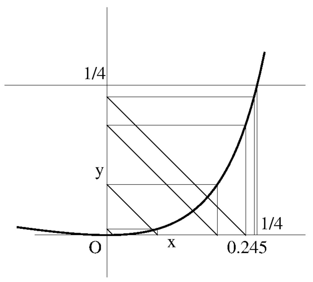
If a starting value of $x = a.b$ is selected somewhere inside the interval
$0 \le x < 1/4$, and it does not coincide with the point $1/4$, then it
is observed that the successive iterates converge (rather quickly) to $x = 0$.
If we commit ourselves to modern terminology, then we would say that the point
$x = 0$ is an attractor of the function $y(x) = x^2/(2.x-1)^2$ over the
interval $0 \le x < 1/4$. An enlargement of the function in the neighbourhood
of the attractor is depicted in the figure below. Click On Pic for viewing
the PostScript code:
"Some Stable Solutions" were found in the chapter with the same name, but they
were found regardless of any considerations about a "safe" domain of interest.
Is it a coincidence that the safety condition $a.b \le 1/4$ does not play any
role in this case? Is it perhaps due to the fact that the stability condition
we have adopted instead, is actually stronger than the condition for safety?
Let's see:
$$
a + b \le 1 \hieruit (a + b)^2 \le 1 \hieruit
a^2 - 2.a.b + b^2 \le 1 - 4.a.b
$$ $$
\hieruit 1 - 4.a.b \ge (a - b)^2 \ge 0
$$
Herewith it is demonstrated that Stability is, indeed, a sufficient condition
for Safety. But it should be emphasized, at the same time, that Stability is
not necessary for Safety: there may exist Safe Solutions which are not
Stable.