MultiGrid

A possible implementation of the Newton-Raphson method for linear equations is triggered by the following observation. Consider a one-dimensional grid:

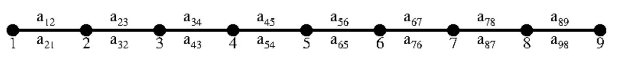
Then, in almost all cases, only adjacent grid-points will be connected by certain (matrix) coefficients. This gives rise to a tri-diagonal system of equations. Let's assume beforehand that the equations are always normed (which means that the elements of the main diagonal must be non-zero from the start). Thus, without loss of generality, we may assume: $$ A = \left[ \begin{array}{ccccccccc} 1 & a_{12} & & & & & & & \\ a_{21} & 1 & a_{23} & & & & & & \\ & a_{32} & 1 & a_{34} & & & & & \\ & & a_{43} & 1 & a_{45} & & & & \\ & & & a_{54} & 1 & a_{56} & & & \\ & & & & a_{65} & 1 & a_{67} & & \\ & & & & & a_{76} & 1 & a_{78} & \\ & & & & & & a_{87} & 1 & a_{89} \\ & & & & & & & a_{98} & 1 \end{array} \right] $$ The matrix $M$ is then formed by $M = I - A$: $$ \left[ \begin{array}{ccccccccc} 0 & -a_{12} & & & & & & & \\ -a_{21} & 0 & -a_{23} & & & & & & \\ & -a_{32} & 0 & -a_{34} & & & & & \\ & & -a_{43} & 0 & -a_{45} & & & & \\ & & & -a_{54} & 0 & -a_{56} & & & \\ & & & & -a_{65} & 0 & -a_{67} & & \\ & & & & & -a_{76} & 0 & -a_{78} & \\ & & & & & & -a_{87} & 0 & -a_{89} \\ & & & & & & & -a_{98} & 0 \end{array} \right] $$ And the matrix $I - M^2$ can be computed. It turns out to be of the form: $$ \left[ \begin{array}{ccccccccc} a_{11} & 0 & a_{13} & & & & & & \\ 0 & a_{22} & 0 & a_{24} & & & & & \\ a_{31} & 0 & a_{33} & 0 & a_{35} & & & & \\ & a_{42} & 0 & a_{44} & 0 & a_{46} & & & \\ & & a_{53} & 0 & a_{55} & 0 & a_{57} & & \\ & & & a_{64} & 0 & a_{66} & 0 & a_{68} & \\ & & & & a_{75} & 0 & a_{77} & 0 & a_{79} \\ & & & & & a_{86} & 0 & a_{88} & 0 \\ & & & & & & a_{97} & 0 & a_{99} \end{array} \right] $$ It is observed now that all even and odd indices have become uncoupled. The variables can be permuted and the equations be rearranged accordingly: $$ \left[ \begin{array}{cccccccccc} a_{11} & a_{13} & & & & | & & & & \\ a_{31} & a_{33} & a_{35} & & & | & & & & \\ & a_{53} & a_{55} & a_{57} & & | & & & & \\ & & a_{75} & a_{77} & a_{79} & | & & & & \\ & & & a_{97} & a_{99} & | & & & & \\ \_ & \_ & \_ & \_ & \_ & \_ & \_ & \_ & \_ & \_ \\ & & & & & | & a_{22} & a_{24} & & \\ & & & & & | & a_{42} & a_{44} & a_{46} & \\ & & & & & | & & a_{64} & a_{66} & a_{68} \\ & & & & & | & & & a_{86} & a_{88} \end{array} \right] $$ The new equations system is of the form: $$ \left[ \begin{array}{cc} A_1 & 0 \\ 0 & A_2 \end{array} \right] $$ 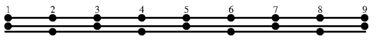Block $A_1$ corresponds with a restriction of the grid to odd-numbered points, block $A_2$ corresponds with a restriction of the grid to even-numbered points, as depicted in the figure below. Such a configuration of coarsened grids will be called a MultiGrid in the sequel.

Once having a blocked system of equations, each block can be solved quite independently of the other. Thus in fact we have two independent systems of equations, $A_1$ and $A_2$, each of them having the same structure as the original system $A$. These equations shall be renormalized at each step, thus assuring that also the new matrices have a diagonal equal to the identity. Probably we can apply the same procedure again and again, thereby reducing any tri-diagonal matrix into ever smaller blocks, which will finally become just single numbers along the main diagonal. After normalization of the latter we should be finished. A well documented implementation of the Newton-Raphson MultiGrid method, programmed in (Turbo) Pascal, is found in Appendix II.