The Hyperbolic Connection

$ \def \EN {\quad \mbox{and} \quad} \def \OF {\quad \mbox{or} \quad} \def \half {\frac{1}{2}} \def \hieruit {\quad \Longrightarrow \quad} \def \slechts {\quad \Longleftrightarrow \quad} $ A Trigonometric Connection has been found for the "dangerous" domain in the space of products of matrix coefficients. But, satisfactory as it is, we were rather interested in a similar theory for the "safe" domain $0 \le a.b \le 1/4$. It is clear that the function $1/a.b=2+2.\cos(\pi.h)$ cannot be used for this domain, not because of its properties for doubling or halving the angle, but because of the fact that its range is limited to $0 \le 1/a.b \le 4$. For the safe domain, a range $0 \le a.b \le 1/4$ or $4 \le 1/a.b < \infty$ would be needed instead. Hence the question is: do there exist functions which have the same properties for doubling and halving their arguments as the trigonometric functions, but also have a quite different range? The answer is yes. These functions do indeed exist. They are called Hyperbolic Functions. As the name already suggests, hyperbolic functions are associated with an (orthogonal) hyperbola, in contrast with the trigonometric functions, which are associated with a circle.
$$ x^2 - y^2 = 1 \quad \OF \quad y(x) = \sqrt{x^2-1} \quad \mbox{for} \quad x \ge 1 $$ An arbitrary area underneath $y(x)$ can be calculated with help of the integral: $ \int_{1}^x y(t) \, dt $. Let's invoke a little help from MAPLE:

int{sqrt(t^2-1),t=1..x);

Then we find: $$ \int_{1}^x y(t) \, dt = \half x \sqrt{x^2-1} - \half \ln \left( x + \sqrt{x^2-1} \right) $$

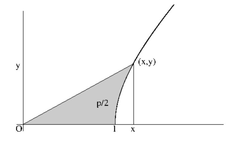
The first term in this expression is the area of a triangle with base $x$ and height $y$. The expression as a whole represents the area underneath $y$ from $1$ to $x$. Thus the second term in the expression represents the area which is spanned by the x-axis, a vector from the Origin to $(x,y)$ and the curved line between $(1,0)$ and $(x,y)$. The latter area may be taken as an analogy with the area $\phi/2$ within a (unit-)circle sector. Hence we could make the following choice, when defining a "hyperbolic angle" $2.p/2$ instead of $2.\phi/2=\phi$: $$ p = \ln \left( x + \sqrt{x^2-1} \right) = \ln(x+y) $$ Herewith we define a hyperbolic sine and a hyperbolic cosine: $$ \sinh(p) = y \qquad \cosh(p) = x $$ And a hyperbolic tangent, eventually: $$ \tanh(p) = \frac{\sinh(p)}{\cosh(p)} $$ It is possible to find explicit expressions for the hyperbolic functions: \begin{eqnarray*} p = \ln(x+y) \hieruit x + y = e^{+p} \\ x^2 - y^2 = 1 \hieruit (x + y)(x - y) = 1 \hieruit x - y = e^{-p} \end{eqnarray*} Addition and subtraction, or solving the equations for $x$ and $y$ gives: $$ \sinh(p) = \frac{e^{+p} - e^{-p}}{2} \qquad \cosh(p) = \frac{e^{+p} + e^{-p}}{2} \qquad $$ And, eventually: $$ \tanh(p) = \frac{e^{+p} - e^{-p}}{e^{+p} + e^{-p}} $$ The following formula is the hyperbolic analogy of $\cos^2(x)+\sin^2(x)=1$ : $$ \cosh^2(p) - \sinh^2(p) = 1 \hieruit \cosh^2(p) - 1 = \sinh^2(p) $$ Especially the function $\cosh(p)$ will be of interest to us. It is immediately clear that the range of $\cosh(p)$ is precisely the kind of completion which is needed for the "safe" domain of interest: $$ 1 \le \cosh(p) < \infty \qquad \mbox{while} \qquad -1 \le \cos(\pi.h) \le +1 $$ Where the minimum value is attained as $\cosh(0) = 1$. It is questioned now if formulas for doubling or halving the hyperbolic angles do indeed exist: $$ \cosh(2.p) = \frac{e^{+2.p} + e^{-2.p}}{2} = \frac{ \left( e^{+p} \right)^2 + \left( e^{-p} \right)^2 + 2.e^{+p}.e^{-p} - 2}{2} = $$ $$ 2 \left(\frac{ e^{+p} + e^{-p}}{2}\right)^2 - 1 = 2.\cosh^2(p) - 1 \hieruit $$ $$ \cosh(2.p) = 2.\cosh^2(p) - 1 \EN \cosh(\half p) = \sqrt{ \frac{1 + \cosh(p)}{2} } $$ Doubling the grid-spacing corresponds with doubling the hyperbolic angle, while halving the grid-spacing corresponds with halving the hyperbolic angle, meaning that the hyperbolic angle must be proportional to the grid-spacing: $$ p = Q.dx \quad \mbox{with} \quad Q \ge 0 $$ The latter condition imposes no limitation on generality, because the hyperbolic cosine is symmetric: $\cosh(p)=\cosh(-p)$. Therefore the absolute value of its argument is all that matters. Thus $Q$ is a positive constant which eventually has to be determined later on. The hyperbolic cosine is ready to take over now where the trigonometric cosine has failed. As with the trigonometric cosine, we shall propose: $$ a.b(dx) = \frac{1}{2 + 2.\cosh(Q.dx)} $$ All persistent properties will remain the same, because they are only dependent upon the formulas for doubling and halving. And with respect to these formulas it makes no difference whether we use the trigonometric or hyperbolic connection. It may be even remarked that the trigonometric and the hyperbolic connection are transformed in each other at $(1/4,1/4)$, by switching from an imaginary to a real argument, or vice versa, because: $$ \cosh(j.\phi) = \frac{e^{+j.\phi} + e^{-j.\phi}}{2} = \cos(\phi) \qquad \mbox{where} \quad j = \mbox{ imaginary unit} $$ The above formula for $a.b(dx)$ can be written in a more transparent form: $$ a.b(dx) = \frac{1}{2 + 2.\cosh(Q.dx)} = \frac{1}{2+2.\left[2.\cosh^2(Q/2.dx)-1\right]} $$ Resulting in: $$ a.b = \frac{1/4}{\cosh^2(Q/2.dx)} \hieruit \sqrt{a.b} = \frac{1/2}{\cosh(Q/2.dx)} $$ From the preceding paragraph, we also have: $$ \frac{b}{a} = e^{P.dx} \hieruit \sqrt{ \frac{b}{a}} = e^{P/2.dx} \EN \sqrt{ \frac{a}{b}} = e^{-P/2.dx} $$ It is a simple matter now to find the explicit formulas, relating each of the off-diagonal coefficients to the distances $dx$ in the grid: \begin{eqnarray*} b = \sqrt{\frac{b}{a}} \sqrt{a.b} = \frac{\half e^{+P/2.dx}}{\cosh(Q/2.dx)} = \frac{e^{+P/2.dx}}{e^{+Q/2.dx} + e^{-Q/2.dx}} \\ a = \sqrt{\frac{a}{b}} \sqrt{a.b} = \frac{\half e^{-P/2.dx}}{\cosh(Q/2.dx)} = \frac{e^{-P/2.dx}}{e^{+Q/2.dx} + e^{-Q/2.dx}} \end{eqnarray*} Herewith a new light is shed upon all kind of persistent properties. For example: $$ a + b = \frac{e^{+P/2.dx}}{e^{+Q/2.dx} + e^{-Q/2.dx}} + \frac{e^{-P/2.dx}}{e^{+Q/2.dx} + e^{-Q/2.dx}} = $$ $$ \frac{e^{+P/2.dx} + e^{-P/2.dx}}{e^{+Q/2.dx} + e^{-Q/2.dx}} = \frac{\cosh(P/2.dx)}{\cosh(Q/2.dx)} $$ It is seen therefrom that the following relationships are true: \begin{eqnarray*} a + b < 1 \slechts | P | < | Q | \\ a + b = 1 \slechts | P | = | Q | \\ a + b > 1 \slechts | P | > | Q | \end{eqnarray*} The absolute values come from: $\cosh(-P.dx)=\cosh(P.dx)=\cosh(|P|.dx)$.
Another interesting quantity is the so-called matrix discriminant, for which the sign was found to be persistent. Meanwhile the sign has even become positive, because of $a.b\le 1/4$ and: $$ 1 - 4.a.b = 1 - 4 . \frac{1/4}{\cosh^2(Q/2.dx)} = \frac{\cosh^2(Q/2.dx)-1}{\cosh^2(Q/2.dx)} $$ $$ = \frac{\sinh^2(Q/2.dx)}{\cosh^2(Q/2.dx)} = \tanh^2(Q/2.dx) $$ Let's try now for even more general solutions of the finite difference equation which is accompanying the tri-diagonal system of equations: $$ - b . T_{i-1} + T_i - a . T_{i+1} = 0 $$ Solutions of the form $T_i = K^{i-1}$ will be attempted. Substitution leads to: $$ K^{i-2} \left[ - b + K - a.K^2 \right] = 0 \OF a.K^2 - K + b = 0 $$ A real-valued solution exists iff the discriminant $1 - 4.a.b \ge 0$. Since the discriminant equals $\tanh^2(Q/2.dx)$, there is no question about it. Substitute now the expressions that we have found for $a$ and $b$, giving: $$ e^{-P/2.dx}.K^2 - \left( e^{+Q/2.dx} + e^{-Q/2.dx} \right) K + e^{+P/2.dx} = 0 $$ $$ K^2 - e^{P/2.dx} \left( e^{+Q/2.dx} + e^{-Q/2.dx} \right) K + e^{P.dx} = 0 $$ $$ \left( K - e^{(P+Q)/2.dx} \right) \left( K - e^{(P-Q)/2.dx} \right) = 0 $$ Resulting in: $$ T_i = \lambda . K_1^{i-1} + \mu . K_2^{i-1} \qquad \mbox{with} \quad K_1 = e^{(P+Q)/2.dx} \EN K_2 = e^{(P-Q)/2.dx} $$ At last, $(i-1).dx$ can be simply replaced by $(x)$, yielding the equivalent: $$ T(x) = \lambda . e^{(P+Q)/2.x} + \mu . e^{(P-Q)/2.x} $$ Which, at the same time, is recognized as a general Analytical Solution.