This paper is the third one in a series of articles about the Variable Mass theory.
Earlier publications in the VM series are: 1. Atomic Time, Orbital Time and the Variable Mass Theory and 2. The Variable Mass Theory and Gravitational Paradoxes. The main content of the first two papers is supposed to be more or less familiar to the reader.
Length Contraction is a feature of Variable Mass. It will be argued that Length Contraction with VM is observationally equivalent with the expansion of Empty Space. In this way a couple of mathematical tools that are useful for our theory can be outsourced to the (nowadays common) expanding universe model.
Conditions are investigated for which a Static Euclidean Universe has a radius larger than the Schwarzschild Radius. We find that a SEU with constant non-zero mean mass density can only exist if it is finite.
As Variable Mass is entering the stage, the playground becomes completely different. Especially relevant is the discovery of an Observability function fO(x). Giving rise to an Observable Universe, which more lucidly may be called a Black Hole Bubble, because it moves through cosmos along with the observer in its center.
A value for the radius of the Black Hole Bubble is calculated. This value is reasonably close to the radius of the Observable universe as accepted by the mainstream. It turns out that there is an absolute maximum of 28.5 for the intrinsic cosmological redshift.
The paper is finished with a solution for Olbers' paradox. For a universe without a Big Bang especially the latter is desperately needed.
CONTENTS
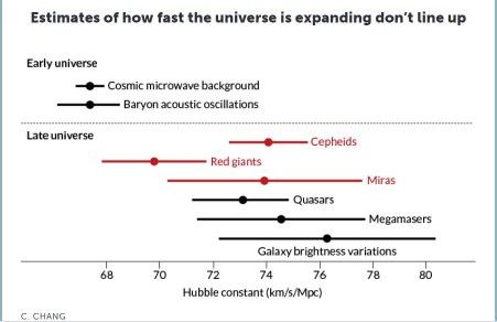
The mathematical machinery in this paper may be rather complicated, but it all rests on one basic formula in [1], namely (9). $$ \frac{m}{m_0} = \large e^{H.t} \normalsize \quad \mbox{with} \quad H = \frac{2}{A} $$ where $m=$ mass, subscript $_0=$ here and now, $H=$ (intrinsic) Hubble parameter, $t=$ atomic time. According to formula (11) in [1] the Hubble parameter is equivalent with twice the inverse of an age $\,A\,$, as measured in the Orbital timeframe. So there is no a priori reason why ages should be equal for the Cosmic microwave background, Red giants, Cepheids, Quasars, the Solar System, the Earth. In VM cosmology the so-called Hubble tension may be essential, instead of something that needs a remedy. This paper is about the (observable) universe as a whole. This means that the Hubble parameter is business as usual, namely $H\equiv H_0\,$, with tensions eventually, as depicted in the figure below.
Likewise it is assumed that the intergalactic medium (IGM) is so much empty that $c\equiv c_0\,$, at a cosmic scale, is the speed of light in vacuum.
Another aspect of the above formula is that distances $\,r\,$ in deep space are measured by light years, not seconds. And (atomic) time is running backwards, because we are looking into the past. This replaces the above formula by an equivalent that will be used throughout this paper, $c=$ speed of light in empty space.
$$
r = c\cdot(-t) \quad \Longrightarrow \quad \frac{m}{m_0} = \large e^{-H/c\,\cdot\,r} \normalsize \qquad (1)
$$
The cosmological redshift $z$ is intrinsic: it only depends on variable (elementary particle rest) mass. Because that is where the VM theory has been designed for:
$$
1+z=\frac{m_0}{m}=\large e^{H/c\,\cdot\,r} \normalsize \qquad (2)
$$
2. Length Contraction
The Compton wavelength [11] of a particle is equal to the wavelength of a photon whose energy $E$ is the same as the rest mass energy of that particle. For a particle here and now it is given by
$$
E_0 = h\nu_0 = h\frac{c}{\lambda_0} = m_0c^2 \quad \Longrightarrow \quad \lambda_0 = \frac{h}{m_0\,c}
$$
where $\nu$ = frequency, $h=$ Planck constant, $c=$ speed of light, $\lambda=$ wavelength, $m=$ (variable) mass.
Suppose again that the Variable (elementary particle rest) Mass will be different / smaller in its own past / larger in its own future, say with a value $m$. Then we have for the Compton wavelength $\lambda$ at that time:
$$
\lambda = \frac{h}{m\,c} = \frac{m_0}{m} \frac{h}{m_0\,c} \\ \Longrightarrow
\quad \lambda = \frac{m_0}{m} \lambda_0
$$
The Compton wavelength ("size") of an elementary particle is inversely proportional with its (varying rest) mass.
Closely related to this is the De Broglie wavelength [12], which is also inversely proportional to elementary particle (rest) mass:
$$
\lambda = \frac{h}{mv}
$$
And the photon wavelength, where the mass $\,m\,$ is not a rest mass, and yet
$$
mc^2 = h\nu = \frac{hc}{\lambda} \quad \Longrightarrow \quad \lambda = \frac{h}{mc}
$$
The Bohr radius [13] is $1/\alpha \approx 137$ times the Compton wavelength (of an electron), where $\alpha$ is the fine structure constant. It is a measure for the size of a hydrogen atom. Let $\,a_0\,$,$\,m_0\,$ be the values of the Bohr radius and (electron rest) mass here and now. And let $\,a\,$,$\,m\,$ be their values at some (proper) time in the past or future. Then it is clear that
$$
a = \frac{1}{\alpha} \frac{h}{mc} \quad \Longrightarrow \quad a = \frac{m_0}{m} a_0
$$
The (Bohr) radius of an (hydrogen) atom is also inversely proportional with varying elementary
particle rest mass (of the electron).
According to [1], not only the Bohr radius, but all real (sub)atomic distances $r$ are found by multiplying dimensionless ones with a Compton wavelength. Therefore they are all inversely proportional to mass. This is expressed by (3) in [1].
$$
\frac{r}{r_0} = \frac{m_0}{m} \quad \mbox{with} \quad m \gt m_0
$$
where $r=$ atomic distance, $m=$ increasing variable (elementary particle rest) mass, subscript $_0=$ here and now.
If an electron jumps between orbits of an atom, then that event is accompanied by an emitted or absorbed amount of electromagnetic energy, commonly called a photon, with frequency $\nu\,$. For a precise motivation, the reader is referred to the sections 1,2,3 in [1].
$$
h\nu = E_1 - E_2 = mc^2\times\mbox{(dimensionless function)}
$$
where $h=$ Planck constant, $E=$ energy levels, $m=$ mass, $c=$ speed of light in vacuum.
Combining the two formulas gives
$$
\frac{h\nu}{h\nu_0} = \frac{mc^2}{m_0c^2} \quad \Longrightarrow \quad \frac{\nu}{\nu_0} = \frac{m}{m_0}
$$
Wavelengths $\lambda$ are often more convenient here than frequencies. With $\nu=c/\lambda$ we get formula (4) in [1]:
$$
\frac{\lambda}{\lambda_0} = \frac{m_0}{m} \quad \mbox{with} \quad m \gt m_0
$$
Wavelengths of light are inversely proportional with (increasing rest) mass (of electrons).
The Electromagnetic Mass [14] of an electron may be calculated as follows. The energy density in an electric field is given in general by $\, w = \frac{1}{2} \epsilon_0 E^2 \,$ where the field strength $\, E \,$ at a distance $\, r\, $ is: $$ E = \frac{q}{4 \pi \epsilon_0 r^2} $$ with $\,q\,$ the electron charge and $\,\epsilon_0\,$ the dielectric constant of the vacuum. The total energy in the field is thus given by $$ U = \int_0^\infty\frac{1}{2}\epsilon_0 \left(\frac{q}{4\pi\epsilon_0 r^2} \right)^2 4 \pi r^2 dr \ = \\ \frac{q^2}{8 \pi \epsilon_0} \int_0^\infty \frac{dr}{r^2} = \infty $$ Thus, in principle, there is an infinite outcome for the rest energy of the electron. Alternative calculations with a finite outcome are feasible though, such as in an article at the Mathematics forum named Cauchy distribution instead of Coulomb law? [16]. The following would have helped in understanding: $$ \int_0^\infty \frac{r^2 dr}{(r^2+\sigma^2)^2} = - \frac{1}{2} \int_0^\infty r\;d\left(\frac{1}{r^2+\sigma^2}\right) \\ = \left[-\frac{r}{2(r^2+\sigma^2)}\right]_{r=0}^\infty + \frac{1}{2\sigma}\int_0^\infty \frac{d(r/\sigma)}{1+(r/\sigma)^2} \\ = \frac{1}{2\sigma}\left[\,\arctan(r/\sigma)\,\right]_{r=0}^\infty = \frac{\pi}{4\sigma} $$ Because now it's easy to see that: $$ U = \frac{q^2}{8 \pi \epsilon_0} \int_0^\infty \frac{r^2 dr}{(r^2+\sigma^2)^2} = \frac{q^2}{4 \pi \epsilon_0}\frac{\pi}{8\sigma} = mc^2 \quad \Longrightarrow \quad \sigma = \frac{\pi}{8}\times\frac{1}{4 \pi \epsilon_0} \frac{q^2}{m c^2} $$ In all cases, since the Classical electron radius $r_e$ [17] is inversely proportional to the electron rest mass, the Length Contraction law holds, by whatever means the "true" radius $\,\sigma\,$ will be calculated: $$ r_e = \frac{1}{4 \pi \epsilon_0} \frac{q^2}{m c^2} \quad ; \quad \sigma \sim r_e \quad \Longrightarrow \quad \sigma = \frac{m_0}{m} \sigma_0 $$ Now it's not such a great step to generalize the above results accordingly:
Wavelengths of electromagnetic radiation, sizes of elementary particles, atoms and molecules are inversely proportional with varying elementary particle (rest) mass.
This result is even more general. A rod or a rope is built from molecules and molecules are built from atoms. These atoms have sort of a Bohr radius. If the Bohr radius changes, then it may be expected that the length of the rod or the rope is changing as well, inversely proportional with the (varying rest) mass of the particles it is made from. Thus all lengths $L$ of things built from molecules or atoms close enough together - solid or fluid material - obey the law of length contraction: $$ \large \boxed{L = \frac{m_0}{m} L_0} $$ It is clear that if length contraction applies to lengths measured with a measuring rod and if the measuring rod itself has become longer as well, then it's impossible to tell the difference between two measurements. Much like in Special Relativity, there is no a priori reason why this sort of length contraction would be inconsistent with observation.
Last but not least: it's reasonable to assume that distances in empty space do NOT show any sort of length contraction.
This has a remarkable consequence. Any length that is bound to matter, whether that is a (measuring) rod or a light ray cast back and forth to the moon, obeys the following law. The length of a length-measuring-device is inversely proportional to varying rest mass: $\,L/L_0 = m_0/m\,$. However, there do not exist other measuring devices than those bound to matter in such a way. But then we must necessarily conclude that any length that is measured by a rod, or by a light ray cast back and forth is observed as being directly proportional to varying rest mass, provided that the length that is measured does not itself change with varying rest mass, which is the same as saying that the latter is not material. This leads to the following important conclusion.
Length Contraction with VM is observationally equivalent with the Expansion of Empty Space.
3. Outsourcing to ΛCDM
Let us repeat how John Michell / Pierre Simon Laplace [18] have arrived at the possible existence of Black Holes. A black hole, or rather a Dark star (Newtonian mechanics) [19] is defined as a body from which no light can escape. It is anyway assumed that our Observable universe [20] is not a Black Hole. The minimal radius $R$ of it is then calculated with the law kinetic energy > potential energy for light particles. According to classical mechanics, with $m=$ mass of a photon:
$$
\frac{1}{2} mc^2 \gt \frac{GM\cdot m}{R} \quad \Longrightarrow \quad R \gt \frac{2GM}{c^2} \qquad (3)
$$
where $G=$ gravitational constant, $M=$ total mass of the body, $c=$ lightspeed. The rightmost quantity is known from General Relativity as the Schwarzschild radius [21]. The above classical derivation is only a heuristic; it must not be considered as a rigorous proof. Like in GR it will be assumed that an object (like cosmos) with a radius smaller than the $2GM/c^2$ cannot have a stable existence.
According to one of our basic assumptions in the Introduction, the mass density $\rho_c$ in the SEU is uniform. In addition, it is assumed constant here. Then we have with Mass = density x (volume of sphere):
$$
R \gt 2GM/c^2 \quad \mbox{with} \quad M = \rho_c\frac{4}{3}\pi R^3 \\
1 \gt 2G.\rho_c\frac{4}{3}\pi R^2/c^2 \\
\rho_c \lt \frac{3}{8\pi}\frac{c^2}{G R^2}
$$
For an infinite SEU we have $R \to \infty$ and consequently $\rho_c \to 0$ . Leading to an important conclusion:
An infinite Static Euclidean Universe is incompatible with a constant non-zero mass density.
There is a standard formula that relates the Hubble parameter $H$ to the Critical density [26] in the Lambda-CDM model [23]. Quote: A critical density $\,\rho_{crit} [\equiv\rho_c]$ is the present-day density, which gives zero curvature $\,k\,$, assuming the cosmological constant $\,\Lambda\,$ is zero, regardless of its actual value. Substituting these conditions to the Friedmann equation gives $$ \rho_c = \frac{3H^2}{8\pi G} \qquad (4) $$ There exists a nice heuristic of (4) within classical physics. Quoting Google AI it reads: This derivation treats the universe as an expanding spherical cloud of mass where the kinetic energy of the expansion perfectly balances the gravitational potential energy. According to Hubble's law [27], the velocity of the expansion at distance $R$ is $v=HR\,$. $$ \frac{1}{2}mv^2 - \frac{GmM}{R} = 0 \\ v = HR \quad ; \quad M = \rho_c\frac{4}{3}\pi R^3 \\ \frac{1}{2}m(HR)^2 = \frac{Gm\rho_c\frac{4}{3}\pi R^3}{R} \\ \frac{1}{2}H^2\,mR^2 = \frac{4}{3}\pi G\rho_c\,mR^2 \\ H^2 = \frac{8}{3}\pi G\rho_c \qquad (4) $$ At first sight, an expanding universe model is not applicable to our SEU. However, we have learned in section 2 of this paper that Variable Mass goes hand in hand with Length Contraction and - more relevant in the current context: Length Contraction with VM is observationally equivalent with the Expansion of Empty Space.
Thus having motivated the applicability of (4) in VM, let's proceed now with another way of looking at our Static Euclidean Universe with constant critical density.
$$
R \gt \frac{2GM}{c^2} \quad \mbox{with} \quad M = \rho_c\frac{4}{3}\pi R^3 \\
1 \gt \frac{(8/3.\pi\,G \rho_c)R^3}{c^2R} = \left(\frac{H}{c}R\right)^2 \\
R \lt \frac{c}{H}
$$
Conclusion: a Static Euclidean Universe (SEU) with constant mass density can only exist if it is finite
(i.e. a sphere with radius $c/H$ where $H\equiv H_0$).
4. Observability function
How can we arrive at an observable universe within an infinite Static Euclidean Universe? Let's see how it works out with the Variable Mass Theory. The mass density in cosmos is no longer constant but, according to (1) we have an exponential decay. This changes the whole scene.
$$
\frac{m}{m_0} = e^{-H/c\,\cdot\,r} \quad \Longrightarrow \quad \rho = \rho_0\,e^{-H/c\,\cdot\,r}
$$
where $\rho_0$ is the mean mass density at our place, here and now. Instead of $M = \rho.\frac{4}{3}\pi R^3$ we have, with (3):
$$
\frac{2GM}{c^2R} \lt 1 \quad \mbox{with} \quad M = \int_0^R \rho_0\,e^{-H/c\,\cdot\,r}.4\pi r^2.dr \\
\frac{2GM}{c^2R} = \frac{8\pi.G.\rho_0}{c^2R} \left(\frac{c}{H}\right)^3 \int_0^R e^{-H/c\,\cdot\,r} (H/c\cdot r)^2.d(H/c\cdot r)
$$
By introducing dimensionless quantities $\,\xi=H/c.r\,$ and $\,x=H/c\cdot R\,$ much simplification is achieved.
$$
\frac{2GM}{c^2R} = \frac{8\pi.G.\rho_0}{H^2}\frac{1}{x}\int_0^x e^{-\xi} \xi^2.d\xi
$$
The integral is solved by
$$
\frac{d}{d\xi}\left[-e^{-\xi}(\xi^2+2\xi+2)\right] = e^{-\xi}\xi^2 \\
\int_0^x e^{-\xi} \xi^2.d\xi = 2-e^{-x}(x^2+2x+2) \qquad (5)
$$
It all leads to the following outcome.
$$
\frac{2GM}{c^2R} = \left(\frac{8\pi.G.\rho_0}{H^2}\right)\frac{2-e^{-x}(x^2+2x+2)}{x} \lt 1 \qquad (6)
$$
Having adopted features of the ΛCDM model, there is no other choice than (4).
$$
H^2 = \frac{8}{3}.\pi.G.\rho_0 \quad \Longrightarrow \quad \frac{8\pi.G.\rho_0}{H^2} = 3 \\
\frac{2GM}{c^2R} = 3\frac{2-e^{-x}(x^2+2x+2)}{x} \lt 1 \qquad (7)
$$
A dimensionless Observability function $f_O$ is defined by
$$
f_O(x) = \frac{2-e^{-x}(x^2+2x+2)}{x} \qquad (8)
$$
A few values of the function $f_O(x)$ for $\,x\ge 0$ are to be found. Define $\,g(x) = -e^{-x}(x^2+2x+2)\,$. We already know that $\,g'(x)=e^{-x}x^2\,$, according to (5).
$$
f_O(0) = \lim_{x\to 0}f_O(x)=\lim_{x\to 0}\frac{g(x)-g(0)}{x}=g'(0)=0 \\
f_O(x)\cdot x = 2 - 2\frac{1+x+x^2/2}{1+x+x^2/2!+x^3/3!+ \cdots} \\
F_O(0) = 0 \quad ; \quad f_O(x) \ge 0 \quad ; \quad \lim_{x\to \infty}f_O(x) = 0
$$
Determine the maximum of the function and give names: $\,(W,w)\,$ with $\,f_O(W)=w\,$. With help of MAPLE [15]:
f_O(x) := 2*(1-exp(-x))/x-x*exp(-x)-2*exp(-x);
diff(f_O(x),x); s := fsolve(%=0,{x});
assign(s); # x = W

                        s := {x = 3.383634283}

w := 2*(1-exp(-x))/x-x*exp(-x)-2*exp(-x);

                          w := 0.3883945571
Hence the maximum value of the Observability function is given by
$$
f_O(W=3.383634283)=w=0.3883945571 \gt 1/3 \qquad (9)
$$
f_O(x) := 2*(1-exp(-x))/x-x*exp(-x)-2*exp(-x);
fsolve(f_O(x)=1/3,x,0..4);
fsolve(f_O(x)=1/3,x,4..100);
Resulting in: $$ f_O(x) \lt 1/3 \; : \; x \lt x_1 \quad \mbox{or} \quad x \gt x_2 $$ where $x_1=2.096433787\,$, $x_2=5.451457921\,$.
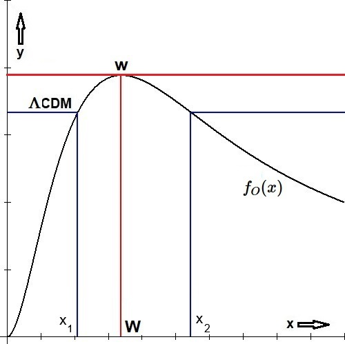
The above result for $f_O(x) \lt 1/3$ turns out to be paradoxical in the end. It would mean for example that objects with distance smaller than $x_1$ can be observed, as well as objects with distance greater than $x_2$, but not in between. So there would be a gap $x_1\lt x \lt x_2$ in our observations. It is reasonable to assume that there are no such "forbidden" Black-Hole-like regions in our observable universe. Apart from this, let's calculate for the cosmological redshift at $x=x_1$. Remember that $x=H/c\cdot r$ with $r=$ "real" cosmic distance. Our formula for intrinsic redshift (2) then becomes
$$
1+z = e^{H/c\,\cdot\,r_1} = e^{x_1} \quad \mbox{with} \quad f_O(x_1) = 1/3
$$
Solving for $x_1=2.096433787$ we find $z=\exp(x_1)-1=7.137099478$ as the maximally observable redshift with the ΛCDM model in our setting. However, quoting Google AI (June 2026): The largest confirmed cosmological redshift observed for a discrete object is for the galaxy MoM-z14. Discovered by the James Webb Space Telescope, it features an extraordinary spectroscopic redshift of $z \approx 14.44$. Which is twice as large. Therefore it must be concluded that the restriction $f_O(x) \lt 1/3$ is in contradiction with observation.
As for the future, it is wise to keep up with the Guinness World Record of the most distant confirmed galaxy in Wikipedia's
List of the most distant astronomical objects [25].
Let's have a second look at our equation (6). Rewrite the condition as follows with (8). $$ f_O(x) \lt \frac{H^2}{8\pi.G.\rho_0} $$ For the maximum (9) of the Observability function we have for sure that $$ f_O(x) \lt w $$ Therefore it's reasonable to declare these two conditions as equivalent. This case corresponds with the red lines in the above figure. $$ \frac{H^2}{8\pi.G.\rho_0} = w \qquad (10) $$ Let the Hubble parameter be the one that is typical for the universe as a whole, say $H\equiv H_0$. Herewith it is assumed that people will agree on the tensions eventually. Quite in general, $H$ is related to the critical density $\rho_0$ of cosmos here and now. For $H$ we have found three different expressions in the past and a fourth one here. For the Schwarzschild Radius the relativistic value $2GM/c^2$ is taken. $G=$ gravitational constant. $$ H^2 = \chi\,8\pi\,G\,\rho_0 \quad \mbox{with} \quad \begin{cases} \chi = 0.3883945571 & (\mbox{d}) \\ \chi = 1/3 & (\mbox{c}) \\ \chi = 1/6 & (\mbox{b}) \\ \chi = 1/8 & (\mbox{a}) \end{cases} $$ Case (a) is derived from formulas (5.7)=(5.12) and (6.12) in [5], case (b) is found as a footnote $\tiny 11$ at page 134 of the book [5], case (c) is compliant to the contemporary standard in cosmology and case (d) has been derived at this place. It is clear that, given an empirical method for determining the Hubble parameter $H$, the critical mass density $\rho_0$ must be different for any of the models (a) thru (d). We have already used the names $\rho_c$ for (b), $\rho_{crit}$ for (c). And now: $\rho_{\tiny \mbox{VM}}$ for (d)? Again, a picture says more than a thousand words.
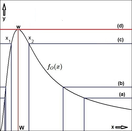
An ascending sequence of cases is observed, where it is seen that the supposed gap in our observations becomes smaller when going from (a) up to (d). We have argued that for case (c) there is a gap $x_1 \lt x \lt x_2$ in our observations. This gap can only be theoretical though. It is not reasonable to calculate the cosmic redshift for $x=x_2$. Likewise we may conclude that it is not reasonable to go beyond the infinitesimal gap that can be thought of at $x=x_1=x_2=W$. The dimensionless number $W$ inevitably must correspond to the maximal distance in our Observable universe [20].
6. Cosmological Redshift
For the radius $R_O$ at the boundary of anyone's Black Hole Bubble we find that
$$
W = \frac{H}{c}R_O \quad \Longrightarrow \quad R_O = 3.383634283 \times (\mbox{Hubble length}) \qquad (11)
$$
Let's calculate [15].
W := 3.383634283;
# Seconds in a year
y := 31556926;
# Speed of light
c := 299792458;
# 1 megaParsec
Mpc := 3.08567758*10^22;
# Hubble parameter (2022-02-08)
H := 73.4*1000/Mpc;
# Radius of Bubble
R_O := c/H*W/(c*y);
                                            11
                      R_O := 0.4507577582 10
# Radius of Bubble
R_O := 46.5*(c*y)*10^9;
# Hubble parameter
H := c*W/R_O;
H := H*Mpc/1000;
                      H := 71.15186981
The first part of our calculation reveals that the radius of the Observable universe is $R_O = 45.1$ billion light-years. Compare this with Wikipedia: The radius of the observable universe is therefore estimated to be about 46.5 billion light-years. The difference between the two outcomes can easily be accounted for by well known Hubble tensions, as is shown in the last part of our calculation: a value of $H=71$ km/s/Mpc does the job.
7. Olbers' Paradox
According to standard (Big Bang) theory an "infinite" universe is impossible. One of the most frequently
employed arguments to defend this stand is Olbers' Paradox (Wikipedia) [7] which is also known as the "dark night sky paradox".
It is the argument that the darkness of the night sky conflicts with the assumption of an infinite
and eternal static universe. In the hypothetical case that the universe is static, homogeneous at a large scale,
and populated by an infinite number of stars, any line of sight from Earth must end at the surface of a star
and hence the night sky should be completely illuminated and very bright. This contradicts the observed
darkness and non-uniformity of the night.
A "line of sight" or rather a ray of light does not really exist in the first place. Even if we adhere
to geometrical optics for simplicity, light still comes to us in thin conical bundles.
A bundle of light rays - departing from a star - is weakening according to the inverse square law for distance.
Stars look fainter as they are farther away.
Common formulations of Olbers' Paradox contain another hidden assumption, namely that the lifetime of stars is
infinite. An essential ingredient of the counter argument is of course that stars are born and stars are dying.
There is a great chance that an outgoing line of sight will meet a place where a light source has not yet been
ignited or meanwhile has extinguished.
The common Big Bang model explains the observed non-uniformity of brightness by invoking
spacetime's expansion, which lengthens the light [ .. ] to microwave levels via a process known as redshift;
this microwave radiation background has wavelengths much longer than those of visible light, and so appears
dark to the naked eye. In this respect, as we have seen, the Big Bang model is not much different from
our version of the Variable Mass Theory [1], as the latter is equipped with Intrinsic Redshift [8]. Thus an analogous argument might be used for debunking Olbers' Paradox,
provided that our intrinsic redshift becomes large enough for the purpose.
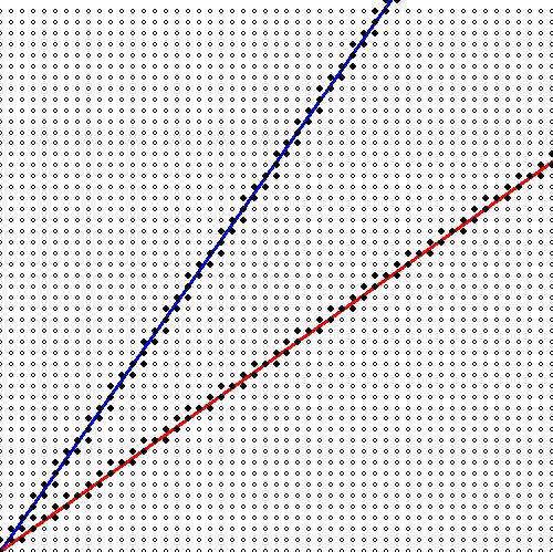 | There is evidence of a more mathematical nature, though, showing that the dark night sky is not a paradox at all. It's a well known fact in mathematics that there exist many more real numbers than there are rational numbers. All rational numbers $y/x$ can be represented by points in a rectangular equidistant grid with integer $(x,y)$ coordinates. The grid points may be considered as stars in a universe, which in our simplified model is 2-D, flat and infinitely large. Starting from the origin, it's easy to draw a (light)ray that passes all stars without hitting any of them. Just define a ray like $\,\color{blue}{y=\sqrt{2}\,x}\,$ or $\,\color{red}{y=x/\sqrt{2}}\,$. It is known that $\sqrt{2}$ is irrational, so it's impossible to have a rational slope $y/x=\sqrt{2}$ or $x/y=\sqrt{2}$ as would be required. Take any irrational number as the slope and it is clear that there are infinitely many more of those rays. |