Atomic Time, Orbital Time
and the Variable Mass Theory
Han de Bruijn, retired Engineer,
Theoretical Physicist by education
E-mail: umumenu@gmail.com
ABSTRACT
Starting with the Hydrogen atom as an example,
a dimensionless formulation of the Schrödinger equation for many electron atoms is presented. It is shown that the energy levels $E$ of such a system are only dependent on the fine structure constant $\alpha$, the atomic number $Z$, the speed of light $c$ in vacuum and elementary particle (rest) masses $m$ of electron and nucleus. If $\alpha$ and $c$ may be assumed to be constants of nature, then $E$ is only dependent on mass $m$. Introducing the Variable Mass hypothesis (VM) leads to formulas for the so-called intrinsic redshift. Ticks of Atomic clocks $\Delta t$ are shown to be inversely proportional to mass $m$.
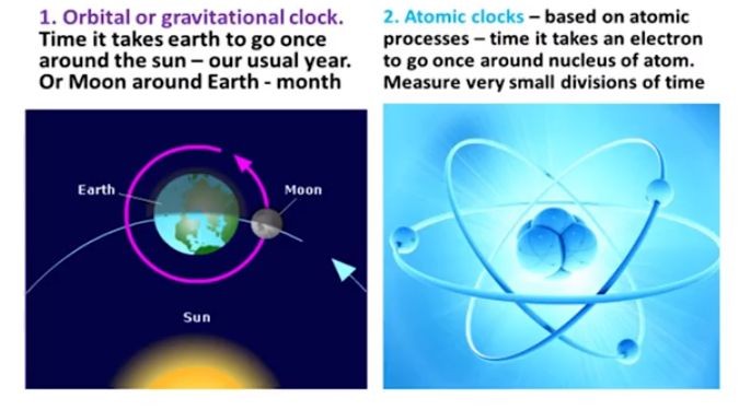
Atomic clocks may seem the most accurate nowadays. Common timing in life, however, is still based upon seconds, minutes and hours, as parts of daylength, and days as parts of a year. This may be called the Orbital timeframe. By considering orbits of planets such as the earth, it is argued that ticks of Orbital clocks $\Delta T$ are inversely proportional to the square root of mass $m$.
If it is accepted that there are two clocks instead of one, then there is a discrepancy between the Atomic ticks $\Delta t$ and the Orbital ticks $\Delta T$, due to Variable Mass. A simple differential equation is derived that relates the two timeframes. For mass in Atomic time $t$, a formula can be derived that shows exponential growth. With help of the differential equation, a formula can be derived for mass in Orbital time $T$ as well, showing quadratic growth and
a beginning for $T=-A$, meaning that there is an age $A$.
Empirical evidence for both the quadratic and exponential growth formulas is found in the Shrinking Kilogram.
Quite unexpectedly, our version of the VM theory is consistent with the infamous C-decay. On the other hand, Variable Mass offers an explanation for the anomalous Earth's Rotation Retardation. At last, it is proved that Leap Seconds cannot be avoided with Atomic time and Orbital time, when combined with the Variable Mass hypothesis. And there is a very simple formula for calculating them.
CONTENTS
- Hydrogen Atom
- Nondimensionalization
- Atomic ticks
- Orbital ticks
- The two Clocks
- Mass in Atomic time
- Mass in Orbital time
- Shrinking Kilogram
- C-decay
- Milne's Formula
- Earth's Rotation Retardation
- Leap Seconds
- References
1. Hydrogen Atom
Hydrogen is the most simple of all atoms. We could try to solve the Schrödinger equation
for its energy levels. But it's much easier to use instead good "old" quantum mechanics, especially the
Bohr model [1] for the atom.
The latter can be considered anyway
as a crude prototype for all atoms. An electron with charge $e$ and mass $m$ describes a circular orbit with radius $r$
and velocity $v$ around a nucleus with the same (opposite) charge. Then with centripetal acceleration and Coulomb's law
we have
$$
m\frac{v^2}{r} = \frac{e^2}{4\pi\epsilon_0 r^2}
$$
where $\epsilon_0$ is the vacuum permittivity.
Quantum Mechanics is entered into the theory by assuming that the circumference of the orbit contains a whole number
$n$ of Matter wave [2] lengths $\lambda$ of the electron:
$$
2\pi r = n\lambda = n\frac{h}{p} = n\frac{h}{mv} \quad \Longrightarrow \quad v=\frac{n\hbar}{mr}
$$
where $p=$ momentum, $\hbar=$ reduced Planck's constant. And so for the radii $r_n$ of the orbits:
$$
r = \frac{e^2}{4\pi\epsilon_0 m v^2} = \frac{e^2 (mr)^2}{4\pi\epsilon_0 m (n\hbar)^2}
$$ $$
1 = \frac{e^2 mr}{4\pi\epsilon_0 n^2 \hbar^2} \quad \Longrightarrow \quad r_n = \frac{4\pi\epsilon_0 n^2 \hbar^2}{e^2 m}
$$ $$
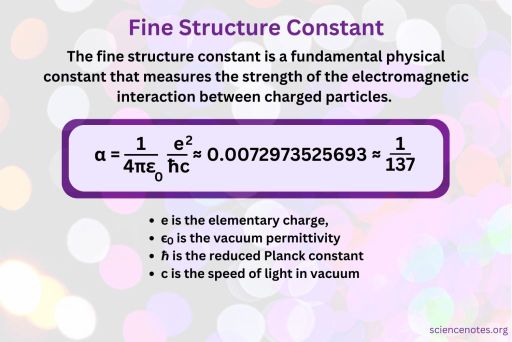
r_n = \frac{4\pi\epsilon_0\hbar c}{e^2}\frac{\hbar}{mc}n^2 = \frac{\hbar}{mc}\mbox{ }\frac{1}{\alpha}\mbox{ }n^2
$$
where $\hbar/(mc)$ is recognized as the Reduced Compton wavelength of the electron and $\alpha$ is the fine-structure constant. In addition, if the Classical electron radius [3] is looked up, the same pattern is observed:
$$
r_e = \frac{\hbar}{mc}\mbox{ }\alpha
$$
The (main) energy levels for hydrogen, at last, are found as follows.
$$
-E_n = \frac{1}{2}mv^2 = \frac{1}{2}\frac{e^2}{4\pi\epsilon_0 r_n}
= \frac{1}{2}\frac{e^2}{4\pi\epsilon_0}\frac{e^2 m}{4\pi\epsilon_0 n^2 \hbar^2}
= \frac{1}{2}\left(\frac{e^2}{4\pi\epsilon_0 \hbar c}\right)^2 mc^2 \frac{1}{n^2}
= mc^2\mbox{ }\frac{\alpha^2}{2}\mbox{ }\frac{1}{n^2}
$$
where $(mc^2)$ is recognized as mass-energy of the electron. Especially take notice of the role played by the Fine Structure Constant $\alpha$:
$$
r_n = \frac{\hbar}{mc}\mbox{ }\frac{1}{\alpha}\mbox{ }n^2 \quad ; \quad
-E_n= mc^2\mbox{ }\frac{\alpha^2}{2}\mbox{ }\frac{1}{n^2}
$$
2. Nondimensionalization
From e.g. Wikipedia we have that the Schrödinger equation for
the Helium atom [4] may be written as
$$
\left[-\frac{\hbar^2}{2m}\nabla_1^2-\frac{\hbar^2}{2m}\nabla_2^2
-\frac{2e^2}{4\pi\epsilon_0 |\vec{r}_1|}-\frac{2e^2}{4\pi\epsilon_0 |\vec{r}_2|}
+\frac{e^2}{4\pi\epsilon_0 |\vec{r}_1-\vec{r}_2|}\right]
\psi(\vec{r}_1,\vec{r}_2) = E\mbox{ }\psi(\vec{r}_1,\vec{r}_2)
$$
Further meaning of symbols:
- $m=$ mass of electron
- $|\vec{r}_{1,2}|=$ distance of electron (1,2) to the nucleus with charge $(2e)$
- $|\vec{r}_1-\vec{r}_2|=$ distance of electron (1) to electron (2)
- $\psi=$ wave function
- $E=$ energy levels (eigenvalues)
For an arbitrary atom - found without a reference / confirmed by Google AI - this may be generalized to
$$
\left[ \sum_{i=1}^Z \left( -\frac{\hbar^2}{2m}\nabla_i^2 - \frac{Ze^2}{ 4\pi\epsilon_0 | \vec{r_i} | } \right) + \sum_{i=1}^Z\sum_{j=i+1}^Z \frac{e^2}{4\pi\epsilon_0 | \vec{r}_i-\vec{r}_j | } \right] \psi(\vec{r}_1,\cdots,\vec{r}_Z) = E\mbox{ }\psi(\vec{r}_1,\cdots,\vec{r}_Z)
$$
where $Z=$ Atomic number [5] and
$$
\vec{r}_i = (x_i,y_i,z_i) \quad \mbox{and} \quad \nabla_i^2 = \frac{\partial^2}{\partial x_i^2} + \frac{\partial^2}{\partial y_i^2} + \frac{\partial^2}{\partial z_i^2}
$$
The technique of Nondimensionalization [6]
shall be applied. Distances $\vec{r}$ are normalized $\rightarrow \vec{\rho}$ with the
Compton wavelength [7] of the electron.
$$
(x,y,z) = \frac{\hbar}{mc}(\xi,\eta,\zeta) \quad \mbox{or} \quad \vec{r} = \frac{\hbar}{mc}\vec{\rho} \qquad (1)
$$ $$
\nabla^2_i(\vec{r}) = \left(\frac{1}{\hbar/mc}\right)^2\left[
\frac{\partial^2}{\partial \xi_i^2} + \frac{\partial^2}{\partial \eta_i^2} + \frac{\partial^2}{\partial \zeta_i^2}\right]
= \left(\frac{mc}{\hbar}\right)^2\nabla^2_i(\vec{\rho})
$$
Herewith we find
$$
\left[-\frac{\hbar^2}{2m}\left(\frac{mc}{\hbar}\right)^2\sum_{i=1}^Z\nabla^2_i(\vec{\rho})
-\frac{mc}{\hbar}\frac{Ze^2}{4\pi\epsilon_0}\sum_{i=1}^Z\frac{1}{|\vec{\rho_i}|}
+\frac{mc}{\hbar}\frac{e^2}{4\pi\epsilon_0}\sum_{i=1}^Z\sum_{j=i+1}^Z\frac{1}{|\vec{\rho_i}-\vec{\rho_j}|}
\right]\psi(\vec{\rho}_i) = E\mbox{ }\psi(\vec{\rho}_i)
$$ $$
mc^2\left[-\frac{1}{2}\sum_{i=1}^Z\nabla^2_i(\vec{\rho})
-Z\frac{e^2}{4\pi\epsilon_0\hbar c}\sum_{i=1}^Z\frac{1}{|\vec{\rho_i}|}
+\frac{e^2}{4\pi\epsilon_0\hbar c}\sum_{i=1}^Z\sum_{j=i+1}^Z\frac{1}{|\vec{\rho_i}-\vec{\rho_j}|}
\right]\psi(\vec{\rho}_i) = E\mbox{ }\psi(\vec{\rho}_i)
$$ $$
\left[-\frac{1}{2}\sum_{i=1}^Z\nabla^2_i(\vec{\rho}) - Z\alpha\sum_{i=1}^Z\frac{1}{|\vec{\rho_i}|}
+\alpha\sum_{i=1}^Z\sum_{j=i+1}^Z\frac{1}{|\vec{\rho_i}-\vec{\rho_j}|}
\right]\psi(\vec{\rho}_i) = \frac{E}{mc^2}\mbox{ }\psi(\vec{\rho}_i) \qquad (2)
$$
According to the Variable Mass Theory [8]
the mass of elementary particles - such as an electron -
varies with cosmic time. It is seen that the dimensionless energies of an arbitrary atom equal $E/(mc^2)$.
Meaning that the real energy levels $E$ of an arbitrary atom are directly proportional to the (variable)
mass $m$, provided that $c=$ constant. This is an essential ingredient of the VM theory.
It must be ensured, however, that all other terms of the dimensionless Schrödinger eigenvalue equation are independent of cosmic time too. The factors of these other terms only contain the atomic number $Z$ and the fine-structure constant $\alpha$. It is thus required that especially the fine-structure constant does not vary with cosmic time. With other words: ${\bf \alpha}$ must be an absolute mathematical constant.
There is an very concise
document
[9] by Hans de Vries, where it is claimed that $\alpha$ is indeed a pure number. Which would mean that $\alpha$ is indeed independent of its (eventually varying) physical constituents.
3. Atomic ticks
According to formula (1), real atomic distances $\left|\vec{r}\right|$
are found by multiplying the dimensionless ones $\left|\vec{\rho}\right|$ with the Compton wavelength of the electron.
And let us assume there is increasing Variable Mass.
Quantities here and now are denoted with a subscript $0$.
$$
\left|\vec{r}\right| = \frac{\hbar}{mc}\left|\vec{\rho}\right|
\quad \Longrightarrow \quad \frac{r}{r_0} = \frac{m_0}{m} \qquad (3)
$$
where the lightspeed $c$ as well as the Planck constant $h$ are supposed to be invariant constants of nature throughout
cosmos. The subscript $0$ denotes here and now.
According to formula (2), the energy levels $E$ of an atom are given in general by a mass-energy factor
times a dimensionless spectral function $S$.
$$
E = mc^2.S(\alpha,Z\alpha,\vec{Q})
$$
where $c=$ lightspeed in vacuum, $Z=$ atomic number, $\alpha=$ fine-structure constant,
$\vec{Q}=$ quantum numbers and, last but not least, $m=$ (inertial) mass, to be more precise:
$$
m = \frac{M m_e}{M + m_e} = \frac{(M/m_e)}{(M/m_e)+1}m_e \approx m_e
$$
with $M=$ mass of nucleus, $m_e=$ mass of electron and $M \gg m_e$. Relativistic effects and nuclear physics have
not been taken into account.
If an electron jumps between orbits, then that event is accompanied by an emitted or absorbed amount of
electromagnetic energy, commonly called a photon [10],
with frequency $\nu$.
$$
h\nu = E_1 - E_2 = mc^2\left[S(\alpha,Z\alpha,\vec{Q_1})-S(\alpha,Z\alpha,\vec{Q_2})\right]
$$
With increasing Variable Mass the quantities here and now are denoted again with a subscript $0$.
$$
h\nu_0 = m_0c^2\left[S(\alpha,Z\alpha,\vec{Q_1})-S(\alpha,Z\alpha,\vec{Q_2})\right]
$$
where $\nu=$ frequency. Combining the two formulas gives
$$
\frac{h\nu}{h\nu_0} = \frac{mc^2}{m_0c^2} \quad \Longrightarrow \quad \frac{\nu}{\nu_0} = \frac{m}{m_0}
$$
The lightspeed $c$ as well as the Planck constant $h$ are supposed to be invariant constants of nature throughout
cosmos. Wavelengths $\lambda$ are often more convenient here than frequencies. With $\nu=c/\lambda$ we have
$$
\frac{\lambda}{\lambda_0} = \frac{m_0}{m} \qquad (4)
$$
Assuming that (elementary particle rest) mass $m$ in the past has been smaller than mass $m_0$ here and now,
we see that all wavelengths $\lambda$ as received from the past are larger than wavelengths $\lambda_0$
here and now. This is called Cosmological Redshift [11]. Expressed into common $z=$ redshift notation:
$$
z = \frac{\lambda-\lambda_0}{\lambda_0} = \frac{\lambda}{\lambda_0} - 1
\quad \Longrightarrow \\ 1+z = \frac{m_0}{m} \qquad (5)
$$
The fact that redshift here is caused by a change of mass inside atoms has given rise to the name Intrinsic
Redshift.
Now suppose that we are building an Atomic clock [12]
instead of observing galaxies. Then the frequency or rather the periods / Atomic ticks $\Delta t$ of the clock are
a more relevant quantity than wavelength. The two are intimately related though.
$$
\lambda = c.\Delta t \quad \Longrightarrow \\ \frac{\lambda}{\lambda_0} =
\frac{\Delta t}{\Delta t_0} = \frac{m_0}{m} \qquad (6)
$$
Therefore, according to VM, atomic clock ticks have been larger / dilated in the past. Such is in concordance with
the Time Dilated Past [13] theory by Mike Helland.
4. Orbital ticks
Not quite long ago, there was the good old definition of the Second [14]
as a Fraction of an ephemeris year [15],
defined by a fixed number of seconds (31 556 926) in a year, together with certain restrictions on the "here and now".
What if we had still adopted this Orbital time as the "true" time nowadays, combined with our Variable Mass Theory?
Classical Orbital Mechanics is relevant in this context, especially the theory of
Elliptical orbits [16].
The Orbital period [17] $\Delta T$ of a body traveling through an elliptic orbit can be computed as
$$
\Delta T = 2\pi\sqrt{\frac{r^3}{\mu}} \quad \mbox{with} \quad \mu = GM
$$
where $r=$ the orbit's semi-major axis, $G=$ gravitational constant, $M=$ mass of the more massive (attracting) body.
Let $M=$ mass of our sun and $r=$ distance between the sun and the earth, then $\Delta T$ cannot be anything else than a year.
Very much the same outcome can be reproduced though by a far simpler model, assuming a circular orbit instead of an elliptical one.
With (centripetal force = gravitational force) we have, for the angular velocity $\omega = 2\pi/\Delta T$ and a circle with radius $r$. The latter is assumed constant for all time.
$$
m \omega^2 r = \frac{GMm}{r^2} \quad \Longrightarrow \quad \Delta T = 2\pi \sqrt{\frac{r^3}{GM}}
$$
Of interest to us is only the (increasing) mass $M$. We see that, in general, there is sort of a Time Delayed Past for Orbital ticks too, which is however different from the one for Atomic clocks, namely
$$
\frac{\Delta T}{\Delta T_0} = \sqrt{\frac{M_0}{M}} = \sqrt{\frac{m_0}{m}} \qquad (7)
$$
It should be noticed that the condition ($r=$ constant) is a necessary one. With $\omega = 2\pi/\Delta T$ :
$$
\Delta T = 2\pi \sqrt{\frac{r^3}{GM}} \quad \Longrightarrow \quad \omega^2 r^3 = GM
\quad \Longrightarrow \quad \left(\frac{\omega}{\omega_0}\right)^2\left(\frac{r}{r_0}\right)^3 = \frac{m}{m_0} \\
\frac{\Delta T_0}{\Delta T} = \frac{\omega}{\omega_0} = \sqrt{\frac{m}{m_0}} \quad \Longrightarrow \quad
\left(\frac{\omega}{\omega_0}\right)^2\left(\frac{r}{r_0}\right)^3=
\left(\frac{m}{m_0}\right)\left(\frac{r}{r_0}\right)^3=\frac{m}{m_0} \quad \Longrightarrow \quad \frac{r}{r_0} = 1
$$
5. The two Clocks
Asking about the unit of clock time, at least three definitions of the Second have been in use.
And still are. We quote from Wikipedia [14]:
- The second is derived from the division of the day first into 24 hours, then to 60 minutes, and lastly to 60 seconds each (24 × 60 × 60 = 86,400). The definition that is based on 1/86,400 of a rotation of the earth is still used by the Universal Time 1 (UT1) system.
- In 1956, the second was redefined in terms of a year relative to that epoch. The second was thus defined as "the fraction 1/31,556,925.9747 of the tropical year for 1900 January 0 at 12 hours ephemeris time". This definition was adopted as part of the International System of Units in 1960.
- The current and formal definition in the International System of Units (SI) is more precise. The second [...] is defined by taking the fixed numerical value of the caesium frequency, $\Delta \nu_{Cs}$, the unperturbed ground-state hyperfine transition frequency of the caesium 133 atom, to be 91 92 631 770 when expressed in the unit $Hz$, which is equal to $s^{-1}$.
The result is that an Orbital second can be defined in two ways, by 86,400 seconds in a day or by 31,556,926 seconds in a year. We have adopted the latter definition for the Orbital timeframe. The Atomic second is the same as is currently accepted as the "more precise" one. For the sake of clarity, personally I do not think that Atomic time as such is "better" than Orbital time. Anyway in our VM theory we have to consider both timeframes, Orbital and Atomic.
The idea of two clocks is found with several authors.
An exact matching with our own theory is not claimed.
The picture below and corresponding naming by Barry Setterfield [18].
The accompanying formulas relating Orbital clock ticks $\Delta T$ and Atomic clock ticks $\Delta t$ to Variable Mass $m$ have been discovered as the formulas (6) and (7) respectively.
$$
\frac{\Delta t}{\Delta t_0} = \frac{m_0}{m} \quad \mbox{and} \quad \frac{\Delta T}{\Delta T_0} = \sqrt{\frac{m_0}{m}}
$$
In order to be able to proceed, we must assume that Orbital time $T$ and Atomic time $t$ are synchronized at the here and now timestamp. This means human action for setting the clocks:
- Here and now is made the same for both clocks. Formally: $t=0$ if and only if $T=0$ or $t=T=0$.
- The two clock ticks are made equal too for $t=T=0$. Formally: $\Delta T_0 = \Delta t_0$ must be taken care of.
With these two precautions taken, we can derive an important formula in our theory.
$$
\frac{\Delta T}{\Delta T_0} / \frac{\Delta t}{\Delta t_0}
= \sqrt{\frac{m_0}{m}} / \frac{m_0}{m} = \sqrt{\frac{m}{m_0}}
$$
Switching to an "exact" result by taking limits for infinitesimal small clock ticks means obtaining a convenient analytical approximation in reality.
$$
\lim_{\Delta\to 0} \frac{\Delta T}{\Delta t} = \sqrt{\frac{m}{m_0}} \quad \Longrightarrow \\
\frac{dT}{dt} = \sqrt{\frac{m}{m_0}} \quad \mbox{or} \quad \frac{dt}{dT} = \sqrt{\frac{m_0}{m}} \qquad (8)
$$
Giving extremely simple differential equations for $T(t)$ or $t(T)$, in principle. The boundary condition $T=t=0$ must be kept in mind.
6. Mass in Atomic time
A formula (8) has been found for calculating the Variable Mass as a function of Atomic time or as a function of Orbital time, provided that one of the two is known: $m(t)$ or $m(T)$. Up to now we have no idea how to determine one of these. The Atomic time function seems to be the most natural one to start with.
An obvious assumption shall be that the change of (elementary particle rest) mass $m$ is uniform. That is: it does not depend upon the origin $(0)$ of its own (proper) atomic time $t$. Then we have, for equal ticks $\Delta t$:
$$
\frac{m(\Delta t)}{m_0} = \frac{m(2\Delta t)}{m(\Delta t)} = \frac{m(3\Delta t)}{m(2\Delta t)} = \cdots
$$
It is seen that
$$
\frac{m(\Delta t)^2}{m_0^2} = \frac{m(2\Delta t)}{m_0} \quad ; \quad
\frac{m(3\Delta t)}{m_0} = \frac{m(\Delta t)}{m_0}\frac{m(2\Delta t)}{m_0} = \frac{m(\Delta t)^3}{m_0^3}
$$
Quite in general, for a number of increments $=N$:
$$
\frac{m(N\Delta t)}{m_0} = \left(\frac{m(\Delta t)}{m_0}\right)^N
$$
where $N\Delta t = t$ is atomic time itself. And $\Delta t = (t/N)$ for the increments, which are all equal.
The term $m(\Delta t)/m_0$ can be written as unity $(1=m_0/m_0)$ plus its first derivative around $t=0$ times an increment.
$$
\frac{m(\Delta t)}{m_0} = 1 + \left.\frac{d}{dt}\frac{m(t)}{m_0}\right|_{t=0}.\Delta t = 1 + H.\frac{t}{N}
$$
where $H$ is some yet to be determined constant - denoting relative change of mass here and now - with the dimension of $t^{-1}$ or Hertz. Next step:
$$
\frac{m(N\Delta t)}{m_0} = \frac{m(t)}{m_0} = \left(1 + H\frac{t}{N}\right)^N
$$
The result for $N\to\infty$ is a well known limit in mathematics.
$$
\lim_{N\to\infty}\left(1 + \frac{Ht}{N}\right)^N = e^{H.t} \quad \Longrightarrow \\
\frac{m}{m_0} = \large e^{H.t} \normalsize \qquad (9)
$$
Herewith the Atomic time function for Variable Mass has been found, apart from a constant named $H$.
7. Mass in Orbital time
We have found a formula, namely (8), for calculating the VM as a function of Atomic time or as a function of Orbital time, provided that one of the two is known: $m(t)$ or $m(T)$. Meanwhile there is a result for $m(t)$, namely (9), and thus it must be possible to calculate for $m(T)$.
$$
\frac{dT}{dt} = \sqrt{\frac{m}{m_0}} \quad \mbox{and} \quad \frac{m}{m_0} = e^{H.t}
$$
By solving the differential equation:
$$
\frac{dT}{dt} = \sqrt{e^{H.t}} = e^{(H/2)t} \quad \Longrightarrow \quad
T = \int e^{(H/2)t} dt = \frac{2}{H}e^{(H/2)t} + C
$$
Use the boundary condition for $t=T=0$:
$$
0 = \frac{2}{H} + C \quad \Longrightarrow \quad C = - \frac{2}{H}
$$ $$
T = \frac{2}{H}e^{(H/2)t} - \frac{2}{H} \quad \Longrightarrow \quad 1 + \frac{H}{2}T = e^{(H/2)t}
$$ $$
\left(1 + \frac{H}{2}T\right)^2 = e^{H.t}
$$
So we have found a second expression in (our version of) the Variable Mass Theory [8], namely (elementary particle rest) mass as a function of Orbital time.
$$
\frac{m}{m_0} = \left(1+\frac{H}{2}T\right)^2 \qquad (10)
$$
Let's evaluate the result with help of a screenshot from the video [8]. The formula as displayed may be called Narlikar's law.
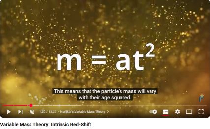
The Variable Mass Theory, according to Jayant Narlikar and Fred Hoyle, is about gravity only. This means that their timeframe is likely to be Orbital. In our notation: $t \rightarrow T$, replace $t$ by $T$ in the first place.
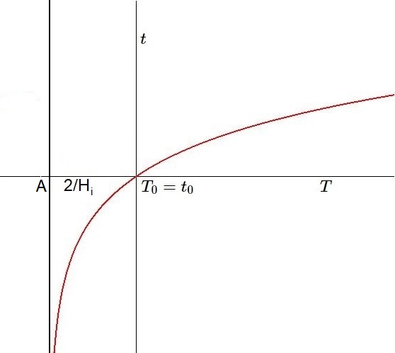
Another issue is their choice of the timestamp $t=T=0$. In the picture by Narlikar and Hoyle, time is set to zero at the timestamp where the "age" of the particle is zero as well as its mass. So let us clarify what the age is in our own formalism for $T=-A$.
$$
\frac{m}{m_0} = 0 \quad \Longleftrightarrow \quad 1+\frac{H}{2}(-A) = 0 \quad \Longleftrightarrow \\
A = \frac{2}{H} \quad \mbox{or} \quad \frac{1}{2}H = \frac{1}{A} \qquad (11)
$$
It follows that Narlikar's law can also be written as
$$
\frac{m}{m_0} = \left(1+\frac{T}{A}\right)^2
$$
And with the differential equations (8) the other way around:
$$
\frac{dt}{dT} = \sqrt{\frac{m_0}{m}} = \frac{1}{1+T/A} \quad \Longrightarrow \quad
t/A = \int dt/A = \int \frac{d(T/A)}{1+(T/A)} = \ln(1+T/A) \\ \Longrightarrow \quad e^{t/A} = 1+T/A
\quad \Longrightarrow \quad e^{H t} = \left(1+\frac{1}{2}H T\right)^2 = \frac{m}{m_0}
$$
where the condition ( $m=m_0 \Longleftrightarrow T=t=0$ ) has been taken into account.
Now take a look at the 1993 publication [19]
by Jayant Narlikar and Halton Arp. Then we find similar results and more. Starting with their formula (8) and converting everything into our own notation (e.g. $t_0\rightarrow A$):
$$
1+z = \frac{t_0^2}{\left[t_0-(r/c)\right]^2} = \frac{A^2}{\left[A-(r/c)\right]^2}
\quad \Longrightarrow \quad \frac{1}{1+z} = \left(1+\frac{T}{A}\right)^2 \quad \mbox{with} \quad r = -c.T
$$
where $r=$ distance. Is that correct within our version of the Variable Mass Theory? Yes it is, because of (5).
$$
H = \frac{2}{A} \quad \mbox{in} \quad \frac{1}{1+z} = \frac{m}{m_0} = \left(1+\frac{H}{2}T\right)^2
$$
Near equation (13) of the Narlikar-Arp paper we quote: expansion of equation (8) gives for small redshifts
$$
z = \frac{2r}{ct_0} , \quad \mbox{i.e. ,} \quad H_0 = \frac{2}{t_0}
$$
Equivalently in our version that would be:
$$
z = \frac{2r}{cA} \quad ; \quad H = \frac{2}{A}
$$
Thus ultimately revealing the meaning of the constant $H$. It is similar to the $H_0$ constant in
Hubble's law [20].
Interesting to notice that - in order to arrive at analogous results as in [19] -
General Relativity is not needed.
GR is effectively replaced by VM. GR has not become invalid, but it's rather redundant for the purpose. Or, as stated in [19]: Finally, the Euclidean, flat spacetime becomes a natural, primary reference frame in which cosmological processes are most simply described. The Variable Mass Theory is compatible with a static Euclidean universe, which is eternal in Atomic time and has moments of creation (i.e. one or more beginnings) in Orbital time.
8. Shrinking Kilogram
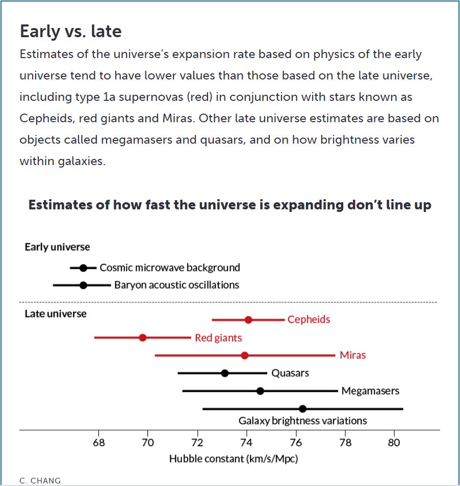
It has been found that $H=H_0=$ the Hubble constant. The benefits of this finding are questionable, because there exists a so-called Hubble tension [20]. Therefore $H_0$ is not so much a constant. It can even be conjectured that every other way of establishing a value for $H_0$ might give rise to different and incompatible outcomes. Therefore a better name for $H$ would be the Hubble parameter.
It has also been found that $A=2/H$, where $A$ is an Age in the Orbital timeframe. But the same $A$ cannot be an Age in Atomic time, as is obvious from the exponential increase in $t$, without a beginning. Summarizing (9), (10), (11):
$$
\frac{m}{m_0} = \left(1+\frac{H}{2}T\right)^2 = e^{H.t} \quad \mbox{with} \quad H = \frac{2}{A}
$$
In case there exists more than one moment of creation - say one for the universe as a whole ($A=28.8$ billion years) and one for the earth in particular ($A=4.9$ billion years) - then there is an issue that resembles the above discrepancies with the Hubble parameter. It seems to be wise to anyway not identify under all circumstances our $H$ with the common $H_0$.
The Hubble parameter is determined from e.g. redshift data, resulting in an estimate for the (gravitational) age of the universe. This sort of knowledge is of course absent if we want to determine the age of the earth. But it's still possible to define a sort of Hubble parameter for the Earth, by employing the above relationship: Age is twice the Hubble time. Let it be so by definition.
But if such is the case with the Earth, why not then with other objects / features in the universe, such as CMB, BAO, Cepheids, Red Giants, Quasars, Megamasers, Galaxies. They all may have different creation timestamps and hence different Hubble parameters.
That being said, we are going to present some direct empirical evidence of Variable Mass on an earthly scale.
From Shrinking Kilogram Bewilders Physicists [21] we quote:
A kilogram just isn't what it used to be. The 118-year-old cylinder that is the international prototype for the metric mass, kept tightly under lock and key outside Paris, is mysteriously losing weight - if ever so slightly.
Were slightly means 50 micrograms. More details are found
elsewhere [22].
According to VM we have, with meaning of the symbols as in previous writings
$$
\frac{m}{m_0} = \left[1+\frac{H}{2}T\right]^2 = \left[1+\frac{T}{A}\right]^2 \approx 1+2\frac{T}{A} \\
\mbox{Alternatively:} \quad \frac{m}{m_0} = e^{H.t} = e^{2t/A} \approx 1+2\frac{t}{A}
$$ $$
\frac{m-m_0}{m_0} \approx \frac{2 \times 118}{4.54 \times 10^9} \approx 52 \times 10^{-9}
$$
Thus $(m-m_0)$ is indeed approximately 50 micrograms when compared with $m_0 = 1\mbox{ }kg$.
Has the standard kilogram really been shrinking? No! Thanks to its splendid isolation it has remained constant all the time. But all matter around it has been suffering from Increasing Mass. Due to its interaction with cosmos [8] the latter has become heavier, with the amount as calculated.
9. C-decay
There is an issue with the theory in the paper by Arp and Narlikar, due to the fact that only one kind of timeflow is recognized, which is Orbital time, also called gravitational time by some. But with our version of the Variable Mass Theory there is also the Atomic timeframe. The (vacuum) speed of light in both timeframes is defined by a distance $dr$ divided by a time increment, in two ways.
$$
c_t = \frac{dr}{dt} \quad \mbox{and} \quad c_T = \frac{dr}{dT}
$$
If it is assumed that the lightspeed in Atomic time is an absolute constant ( i.e. $c_t=c_0$ ) then the lightspeed in Orbital time must be different. Using (8) and (10) we have
$$
c_T = \frac{dr}{dT} = \frac{dr}{dt}\frac{dt}{dT} \quad \mbox{with} \quad
\frac{dT}{dt} = \sqrt{\frac{m}{m_0}} = 1+\frac{H}{2}T \quad \Longrightarrow \quad c_T = \frac{c_0}{1+\frac{H}{2}T}
$$
Therefore the infamous C-decay Theory of Barry Setterfield [23] (take $T\le 0$) is - quite unexpectedly - compatible with (our version of) the Variable Mass Theory.
In the Arp-Narlikar paper a bit more complicated derivation shall be needed for reproducing their formula (13). Of minor importance, because the equivalent result can be proved much easier within the Atomic timeframe, using (5) and (9).
$$
1+z = e^{-H.(-t)} \approx 1+H.t \quad \Longrightarrow \quad z = H.t = H.\frac{r}{c_0} = \frac{2r}{c_0.A}
$$
A far more serious consequence of c-decay is the following though. For $mc^2$ we have conservation of mass-energy in Orbital time, which is the proper timeframe for gravitation.
$$
c_0 = c\sqrt{\frac{m}{m_0}} \quad \Longrightarrow \quad
\frac{m c^2}{m_0 c_0^2} = \frac{m}{m_0}/\frac{c_0^2}{c^2} = \frac{m}{m_0}/\left(\sqrt{\frac{m}{m_0}}\right)^2 = 1
\quad \Longrightarrow \quad mc^2 = m_0c_0^2
$$
Recall the dimensionless formula (2) for the energy levels of an arbitrary atom. And apply conservation of mass-energy in there.
$$
\left[-\frac{1}{2}\sum_{i=1}^Z\nabla^2_i(\vec{\rho}) - Z\alpha\sum_{i=1}^Z\frac{1}{|\vec{\rho_i}|}
+\alpha\sum_{i=1}^Z\sum_{j=i+1}^Z\frac{1}{|\vec{\rho_i}-\vec{\rho_j}|}
\right]\psi(\vec{\rho}_i) = \frac{E}{mc^2}\mbox{ }\psi(\vec{\rho}_i) = \frac{E}{m_0c_0^2}\mbox{ }\psi(\vec{\rho}_i)
$$
Due to Quantum Mechanics, $E$ remains an absolute constant in Orbital time. So there is no Intrinsic Redshift at all, at least not within the pure gravitational framework as designed by Halton Arp & Jayant Narlikar!
10. Milne's Formula
The basic formulas (9),(10),(11) in (our version of) the VM theory can not be repeated frequently enough.
$$
\frac{m}{m_0} = \left(1+\frac{1}{2}H.T\right)^2 = e^{H.t} \quad \mbox{with} \quad H = \frac{2}{A}
$$
where $m=$ mass, $H=$ Hubble parameter, $T=$ orbital time, $t=$ atomic time, $A=$ age. The result can also be written as follows.
$$
\sqrt{\frac{m}{m_0}} \quad : \quad 1+\frac{1}{2}H.T = 1+\frac{T}{A} = e^{(H/2)t} = e^{t/A}
$$
Herewith it's easy to determine $T$ as a function of $t$, and $t$ as a function of $T$.
$$
T = A\left(e^{t/A}-1\right) \quad \mbox{and} \quad t = A\mbox{ }\ln\left(1+\frac{T}{A}\right)
$$
Professor Edward Arthur Milne too has distinguished two kinds of time: ephemeral or dynamical time $\tau$, and absolute or kinematic time $t$, as repeated over and over again in three of his papers:
The relationship between the timeframes $\tau$ and $t$ by Milne is, according to the first reference:
$$
\tau = t_0\mbox{ }\log\left(\frac{t}{t_0}\right)+t_0 \qquad \mbox{(A)}
$$
Compare with our relationship between the timeframes $t$ and $T$.
$$
t = A\mbox{ }\ln\left(1+\frac{T}{A}\right)
$$
Like in the Arp & Narlikar paper, the origin of time is taken as $t_0$ being the present value of the age of the universe at ourselves. With other words: $t_0 = A$. A next correction is renaming of variables and substitution: $\tau \rightarrow t+A$ and $t \rightarrow T+A$, thus bringing the origins of atomic time $t$ and orbital time $T$ back to here and now. Having done all that, there still is a discrepancy between Milne's theory and ours, coming from his physical interpretation of $\tau$ and $t$, which seems to be exactly the other way around!
Anyway, a picture says more than a thousand words.
In a book [27] by
Tom van Flandern [28]
we find in a footnote on page 95 the following.
This formula in the Meta model can be derived with Milne's (modified) formula.
$$
\sqrt{\frac{1}{1+z}}=\sqrt{\frac{m}{m_0}} = 1+\frac{H}{2}T \quad \mbox{with} \quad A = \frac{2}{H}
$$ $$
d = c.(-t) = -c.A\mbox{ }\ln\left(1+\frac{T}{A}\right) = -c\frac{2}{H}\mbox{ }\ln\left(\sqrt{\frac{1}{1+z}}\right)
= -c\frac{2}{H}(-\frac{1}{2})\ln(1+z)
$$ $$
d = \frac{c}{H}\mbox{ }\ln(1+z) \qquad (12)
$$
However, the above derivation with help of Milne's formula is too much of a good thing. If we restrict attention to the Atomic timeframe only, then the proof is reduced to a one-liner by using (5) and (9) again.
$$
1+z=e^{-H.t} \quad \Longrightarrow \quad \frac{H}{c}(-ct) = \ln(1+z) \quad \Longrightarrow \quad d = \frac{c}{H}\mbox{ }\ln(1+z)
$$
It should be noticed that the logarithmic distance formula is not at all restricted to van Flandern's Meta theory. And there are Hubble tensions in $H$, making it possible that there are different intrinsic redshifts $z$ at the same distance $d$.
11. Earth's Rotation Retardation
Let's resume an equivalent of the formulas (9),(10),(11) with $A=$ age.
$$
1+T/A = e^{t/A} \quad \Longleftrightarrow \quad t = A\mbox{ }\ln(1+T/A)
$$
Calculate velocities $v$ and accelerations $a$ from displacements $s$ within the two time frames.
$$
\vec{v}_T = \frac{d\vec{s}}{dT} = \frac{d\vec{s}}{dt}\frac{dt}{dT} = \frac{\vec{v}_t}{1+T/A}
$$ $$
(1+T/A)\vec{v}_T = \vec{v}_t \qquad (13)
$$
It is noticed that results in 9. C-decay are a special case, namely for $\vec{v}_T = c_T$ and $\vec{v}_t = c_0$.
Patiently differentiating further with product rule and chain rule gives
$$
\vec{a}_T = \frac{d^2\vec{s}}{dT^2} = \frac{d}{dT}\left(\frac{d\vec{s}}{dt}\frac{dt}{dT}\right) = \frac{d}{dT}\left(\frac{d\vec{s}}{dt}\right)\frac{dt}{dT} + \frac{d\vec{s}}{dt}\frac{d}{dT}\left(\frac{dt}{dT}\right) =
$$ $$
= \frac{d^2\vec{s}}{dt^2}\left(\frac{dt}{dT}\right)^2 + \frac{d\vec{s}}{dt}\frac{d^2t}{dT^2}
$$
Hence
$$
\vec{a}_T = \vec{a}_t\left(\frac{1}{1+T/A}\right)^2 + \vec{v}_t\frac{-1/A}{(1+T/A)^2}
$$ $$
(1+T/A)^2\,\vec{a}_T = \vec{a}_t - \vec{v}_t/A \qquad (14)
$$
Under earthly circumstances here and now we have that $t=T=0$ and so
$$
\vec{v}_T = \vec{v}_t \\
\vec{a}_T = \vec{a}_t - \vec{v}_t/A
$$
Conclusion: velocities in the two time frames are the same, but accelerations are not.
We continue with a quote from the book Origin of Inertia [29] by Amitabha Ghosh, on page 13: It is now an established fact that the spin motion of the Earth is gradually slowing down, and the magnitude of this secular retardation is about $6 \times 10^{-22}\mbox{ } rad/s^2$. That amount of information is already sufficient.
According to our own theory we have from the above: $\vec{a}_T - \vec{a}_t = - \vec{v}_t/A$. Here $\vec{a}_T$ is the acceleration in Orbital time, $\vec{a}_t$ is the acceleration in atomic time, and $A$ is kind of an age. Due to the non-linear relationship between atomic time $t$ and orbital time $T$ a discrepancy between orbital and atomic accelerations shows up. Regardless of the question which of the accelerations is the "true" one, the difference of the two is a vector in the (opposite) direction of one and the same velocity. Furthermore, all accelerations and velocities are proportional with $R=$ radius of the earth = constant, as required by the implicit use of (7).
Now let the unit vector in tangential direction be defined by
$$
\vec{e}_v = \frac{\vec{v}_t}{|\vec{v}_t|} = \frac{\vec{v}_T}{|\vec{v}_T|}
$$
The velocity (component) at the surface of the earth is simply the (constant) radius of the earth times angular velocity $\omega$.
$$
\left(\vec{v}_t\cdot\vec{e}_v\right) = \left(\vec{v}_T\cdot\vec{e}_v\right) = R\,\omega
$$
The component of the orbital minus atomic acceleration is in tangential direction too and can be nothing else than the radius times a change of the same angular velocity.
$$
\left(\vec{a}_T-\vec{a}_t\cdot\vec{e}_v\right) = R\,\dot{\omega}
$$
It follows that the rotation retardation must be described by
$$
\left(\vec{a}_T-\vec{a}_t\cdot\vec{e}_v\right) = -\left(\vec{v}_t\cdot\vec{e}_v\right)/A
$$ $$
\dot{\omega} = - \omega/A \qquad (15)
$$
Calculation (with MAPLE) using the age of the earth gives
# Age of the earth
age := 4.543*10^9;
# Seconds in a year
year := 31556926;
# Seconds in a day
day := 60*60*24;
# Rotation of the earth
omega := 2*Pi/day;
# Retardation
slower := evalf(omega/(age*year));
We find that the retardation is about $5 \times 10^{-22} \mbox{ } rad/s^2$
12. Leap Seconds
There is a small but positive discrepancy between the Atomic daylength and the Orbital daylength, which is exemplified by the existence of Leap Seconds [30].
Empirical
data are obtained from the Wikipedia reference Δ T (timekeeping) [31]. Quote: The value of $\Delta T$ for the start of 1902 is approximately zero; for 2002 it is about 64 seconds. So the Earth's rotations over that century took about 64 seconds longer than would be required for days of atomic time.
Atomic clocks are running somewhat too fast. Therefore it is necessary to "stop" them once or twice in a year or so (source of picture = Wikipedia).
Let's see if we can reproduce. According to common kinematics we have, after a century of the earth's rotation, for its shortage of radians:
$$
\Delta \theta = \frac{1}{2}\dot{\omega} (\mbox{century})^2
$$
It's a simple matter now to derive with help of (15) the number of leap seconds:
$$
\mbox{leaps} = \frac{\Delta \theta}{2\pi}\times\mbox{day} = \Delta \theta \times \frac{\mbox{day}}{2\pi}
$$
But we are a factor two off:
theta := slower/2*(100*year)^2;
leaps := evalf(theta/(2*Pi)*day);

                         leaps := 34.73137354
There is another way to look at the Leap Seconds problem, which is rather based upon the length of a year instead of the daylength. Let's go back to the original definition of Orbital time as defined by the orbit of the earth around the sun and the basic formulas (9),(10),(11).
$$
1+\frac{1}{2} H T = e^{(H/2)t} \approx 1 + \frac{1}{2}H t + \frac{1}{2}\left[\frac{1}{2}H t\right]^2
$$
Let both the Atomic and Orbital clock be synchronized as usual ($t=T=0$) and let them run free for a century, that is
$$
T = (\mbox{century})_T \quad \mbox{and} \quad t = (\mbox{century})_t
$$ $$
\left(1+\frac{1}{2} H T\right) - \left(1 + \frac{1}{2}H t\right) = \frac{1}{2} H(T-t)
\approx \frac{1}{2}H.\frac{1}{4}H t^2 \quad \Longrightarrow \\
(\mbox{century})_T - (\mbox{century})_t \approx \frac{1}{4}H (\mbox{century})^2
= \frac{1}{2}(\mbox{century})^2/\mbox{age}
$$
It is seen that the Atomic clock over years is again running faster than the Orbital clock. Let's calculate:
leaps := (100*year)^2/(2*age*year);

                         leaps := 34.73137354
Surprisingly, the two leaps are exactly the same. That's the reason why I have shown all the decimals as calculated by the Computer Algebra System.
It is obvious, however, that the two calculations correspond with two different phenomena. The first one describes that there is an additional time leap needed for a rotation of the earth to complete its periods over a day.
The second one describes how atomic clocks are running ahead of orbital clocks, defined e.g. by the earth orbiting around the sun in a year.
Thus the orbital clock is running faster over a year with the same amount
as calculated with daytime! Is that a coincidence? Mathematically speaking: no! It turns out that
the calculation for daytime is actually too much of a good thing. It can be simplified a lot, giving exactly the same outcome as for the time of a year.
$$
\mbox{leaps} = \frac{1}{2} \left[ \left(\frac{2\pi}{\mbox{day}}\right)/\mbox{age} \right] (\mbox{century})^2
\times \left(\frac{\mbox{day}}{2\pi}\right) = \frac{1}{2}(\mbox{century})^2/\mbox{age}
$$
For our leap second this would mean that the outcome $\approx 34.7$ should be taken twice instead of once. Thus improved calculation of the leap interval would reveal that it is about $2\times 34.7 \approx$ 69 seconds.
Remember that observation of the leap interval reveals that it is about 64 seconds.
At last it is clear that the "Age of the Earth" is relevant for the calculations and not the "Age of the Universe", whatever the latter might mean. So what we finally have is leaps $=2\times(\mbox{century})^2/(2\times \mbox{age})$. Unless we have been seduced by wishful thinking, the
conclusion is that leap seconds can be calculated by the following extremely simple formula.
$$
\mbox{leap seconds} = \frac{(\mbox{ seconds in a century })^2}{\mbox{age of the earth in seconds}} \qquad (16)
$$
Acknowledgements: I am grateful to Louis Marmet, Mike Helland and Francois Zinserling for their valuable
comments in the ACG discussions
forum [32].
Conflicts of Interest: The author declares no conflicts of interest.
Funding: This research received no external funding.
13. References
- https://en.wikipedia.org/wiki/Bohr_model
- https://en.wikipedia.org/wiki/Matter_wave
- https://en.wikipedia.org/wiki/Classical_electron_radius
- https://en.wikipedia.org/wiki/Helium_atom
- https://en.wikipedia.org/wiki/Atomic_number
- https://en.wikipedia.org/wiki/Nondimensionalization
- https://en.wikipedia.org/wiki/Compton_wavelength
- https://www.youtube.com/watch?v=T7jVviVBzKs
video: Variable Mass Theory: Intrinsic Red-Shift
- http://www.chip-architect.org/physics/fine_structure_constant.pdf
- https://en.wikipedia.org/wiki/Photon
- https://en.wikipedia.org/wiki/Redshift
- https://en.wikipedia.org/wiki/Atomic_clock
- https://www.youtube.com/watch?v=lVoHmVafTns
video: The theory to REPLACE the Big Bang | Nonexpanding Ep. 8
- https://en.wikipedia.org/wiki/Second
- https://en.wikipedia.org/wiki/Second#Fraction_of_an_ephemeris_year
- https://en.wikipedia.org/wiki/Orbital_mechanics#Elliptical_orbits
- https://en.wikipedia.org/wiki/Orbital_period
- https://barrysetterfield.org/
- https://adsabs.harvard.edu/full/1993ApJ...405...51N
FLAT SPACETIME COSMOLOGY: A UNIFIED FRAMEWORK FOR INTERGALACTIC REDSHIFTS
Jayant Narlikar and Halton Arp. The Astrophysical Journal 405: 51-56, 1993 March 1
- https://en.wikipedia.org/wiki/Hubble%27s_law
- https://pubs.aip.org/physicstoday/Online/20850/Shrinking-Kilogram-Bewilders-Physicists
- https://eu.oklahoman.com/story/news/2007/09/12/shrinking-kilogram-bewilders-physicists/61717049007/
- http://www.alternatievewiskunde.nl/cosmology/cdecay_2007Jellison2.pdf
- https://royalsocietypublishing.org/doi/pdf/10.1098/rspa.1937.0023
- https://royalsocietypublishing.org/doi/pdf/10.1098/rspa.1937.0066
- https://royalsocietypublishing.org/doi/pdf/10.1098/rspa.1937.0087
- Tom van Frandern, Dark Matter, Missing Planets & New Comets. Paradoxes Resolved, Origins Illuminated.
North Atlantic Books, Berkeley, California (1993).
- https://en.wikipedia.org/wiki/Tom_Van_Flandern
- Amitabha Ghosh, Origin of Inertia. Extended Mach's Principle and Cosmological Consequences.
First Published 2000 by Apeiron. 4405, rue St-Dominique, Montreal, Quebec H2W 2B2 Canada. ISBN 0-9683689-3-X
- https://en.wikipedia.org/wiki/Leap_second
- https://en.wikipedia.org/wiki/%CE%94T_(timekeeping)
- https://github.com/orgs/a-cosmology-group/discussions
- https://www.barrysetterfield.org/report/report.html
- https://adsabs.harvard.edu/full/1975ApJ...196..661H
- https://github.com/orgs/a-cosmology-group/discussions/160