Proof of Hyperbola

We have seen that, in the theory of varying elementary particle mass, atomic clock seconds are inversely proportional to mass: $$ \frac{\Delta t}{\Delta t_0} = \frac{m_0}{m} $$ Here $\Delta t=$ atomic clock unit of time, $\Delta t_0=$ the same at some reference time $\,t=t_0$ , $m=$ varying elementary particle mass, $m_0=$ the same at that reference time.
Apart from atomic clocks, there exists gravitational clocks. Gravitational clocks are running at a different speed, namely inversely proportional to mass squared: $$ \frac{\Delta T}{\Delta T_0} = \left(\frac{m_0}{m}\right)^2 $$ Here $\Delta T=$ gravitational clock unit of time, $\Delta T_0=$ the same at our reference time $\,T=T_0$ . Which is at the same time the atomic reference time $\, T_0=t_0$ , because the two types of clocks are being synchronized at that time.
Let analysis start. The quotient $m/m_0$ may be called unit elementary particle mass, for obvious reasons. When looking backwards in time, that unit elementary particle mass is decreasing. Assume that it goes like this:

 m
--- = 1.0  0.9  0.8  0.7  0.6  0.5  0.4  0.3  0.2  0.1
m_0

Furthermore, assume that the observer is using a gravitational clock. Then the (split) seconds, or centuries, or whatever units of that gravitational clock are inversely proportional to the values in the following sequence:

| m |2
|---| = 1.0  0.81  0.64  0.49  0.36  0.25  0.16  0.09  0.04  0.01
|m_0|

But the observer does not know that his time units have been greater in the past; he thinks that they have been equal all the time. What could have been observed, however, is that atomic clocks have been running in a different way. To be more precise: it could have been observed that gravitational and atomic clocks have become running out of sync after some time. Now the question is: how many atomic time units are fitting into one gravitational time unit? Backwards in time, the gravitational time units gradually become greater (thanks to the inversely proportional) than the atomic time units. Thus there are fitting more and more atomic time units into one gravitational time unit. Sober thinking reveals that the amount of fit actually is equal to $(m_0/m)^2/(m_0/m)$ , leading to the following sequence:

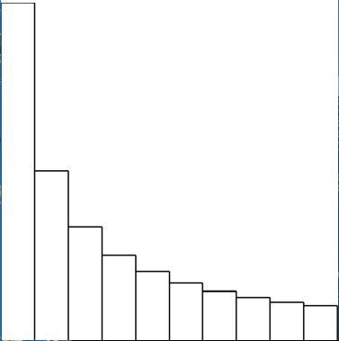
m_0
--- = 1.0  1/0.9  1/0.8  1/0.7  1/0.6  1/0.5  1/0.4  1/0.3  1/0.2  1/0.1
 m

A sequence which has to be read from now (right) towards the past (left). Leading to the following graph:

Refining the calculations with a smaller unit elementary particle mass increase, say $1/100$, leads to the following graph:

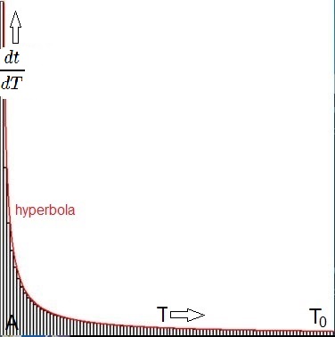
Now it's not difficult to infer that all of these curves converge to an hyperbolic function of the form: $$ \frac{\Delta t}{\Delta T} \to \frac{dt}{dT} = \frac{T_0-A}{T-A} $$ Where $dt$ and $dT$ are the infinitesimal units of atomic time and gravitational time respectively; $T$ is gravitational time; $T_0$ is gravitational reference time, which is the "nowadays" timestamp - rightmost in the graphs - and $A$ is the gravitational timestamp corresponding with the beginning, at the time when mass is created out of nothing - leftmost in the graphs. "General form" means that there is no way to determine the timestamp $A$ theoretically. It must be determined from physical experiments, or by assuming that $A=$ Hubble time from Big Bang theory, or by careful biblical chronology, or whatever.

Mind that the above outcome may sound rather counter-intuitive. That is, because an "easier derivation" may be devised as as follows: $$ \left[ \quad \frac{\Delta t}{\Delta t_0} = \frac{m_0}{m} \quad \wedge \quad \frac{\Delta T}{\Delta T_0} = \left(\frac{m_0}{m}\right)^2 \quad \right] \quad \Longrightarrow \quad \frac{\Delta t}{\Delta T} \to \frac{dt}{dT}= \frac{m}{m_0} = \frac{T-A}{T_0-A} $$ Which is exactly the reverse of the Proof of Hyperbola. This apparent contradiction is explained by the observation that shorter clock ticks - inversely proportional with unit particle mass, squared eventually - correspond with longer time intervals as measured. And the other way around: longer clock ticks correspond with shorter time intervals as measured. So indeed we must have the reverse relationship.
There is another issue: our elementary particle mass seems to be increasing linear with gravitational time. But there are other theories saying that it is quadratric instead.

Still another way of looking at things:

|-------|-------|-------|-------|-------|-------|-------|-------|-------| : t
0123456789012345678901234567890123456789012345678901234567890123456789012
|--------|--------|--------|--------|--------|--------|--------|--------| : T

Suppose the time units of the atomic clock $t$ are $8$ long and the time units of the gravitational clock $T$ are $9$ long. Then: $$ \frac{\mbox{1 unit of t}}{\mbox{1 unit of T}} = \frac{8}{9} $$ However, there are $9$ units of $t$ that fit into $8$ units of $T$ to measure the same time interval of $8 \times 9 = 72$ : $$ \frac{\mbox{#units of t}}{\mbox{#units of T}} = \frac{9}{8} $$

As for Light speed against time, there is no deviation from Setterfield's theory by stating that The graph also represents the rate of ticking of the atomic clock against orbital time [ .. ] The truth of the matter is, these are all the same curve. Moreover it simply follows from the chain rule for differentiation in combination with the definition of the light speed in atomic time units and gravitational time units - $\,ds=$ distance travelled - that the curves are indeed the same (though different from the curves in Setterfield's theory): $$ \frac{c_G}{c_0} = \frac{ds}{dT}/c_0 = \frac{ds}{dt}\frac{dt}{dT}/c_0 = c_0/c_0 \frac{dt}{dT} = \frac{dt}{dT} \quad \Longrightarrow \quad c_G = c_0 \frac{T_0-A}{T-A} $$

Let's consider the Mathematics of radioactive decay (Wikipedia). Given a sample of a particular radioisotope, the number of decay events $-dN$ expected to occur in a small interval of time $dt$ is proportional to the number of atoms present $N$, that is: $$ -\frac{dN}{dt} = \lambda\,N $$ Where $\lambda$ is the decay constant of the particular radionuclide. The solution to this first-order differential equation is: $$ N(t) = N_0\,e^{-\lambda(t-t_0)} = N_0\,e^{-(t-t_0)/\tau} $$ Where $N_0$ is the value of $N$ at time $t=0$.
But results are quite different if gravitational time $T$ instead of atomic time $t$ is taken into account: $$ \frac{dN}{dT}=\frac{dN}{dt}\frac{dt}{dT} = -\lambda\,N\frac{T_0-A}{T-A} \\ \Longrightarrow \quad \int \frac{dN}{N} = -\lambda(T_0-A) \int \frac{dT}{T-A} \\ \Longrightarrow \quad \ln\left(\frac{N}{N_0}\right) = -\lambda(T_0-A) \ln\left(\frac{T-A}{T_0-A}\right) \\ \Longrightarrow \quad N(T) = N_0 \left(\frac{T-A}{T_0-A}\right)^{-\lambda(T_0-A)} \quad \Longrightarrow \\ N(T) = N_0\,e^{-\lambda(t-t_0)} \quad \mbox{with} \quad t-t_0=(T_0-A)\ln\left(\frac{T-A}{T_0-A}\right) $$ The latter expression as expected, because of the known relationship between atomic time and gravitational time: $$ \frac{dt}{dT} = \frac{T_0-A}{T-A} \quad \Longrightarrow \quad t-t_0=(T_0-A)\ln\left(\frac{T-A}{T_0-A}\right) $$

Intervals of the gravitational clock are running proportional to the following sequence, when reading from the right to the left:

|m_0|2
|---| = 1/1.0  1/0.81  1/0.64  1/0.49  1/0.36  1/0.25  1/0.16  1/0.09  1/0.04  1/0.01
| m |

Formally, with $\,\Delta m/m_0 = 1/10$ : $$ \Delta T = \Delta T_0 \left(\frac{m_0}{m}\right)^2 = \Delta T_0 \frac{m_0^2}{(k\,\Delta m)^2} \quad \mbox{with} \quad k = 10,9,8,7,6,5,4,3,2,1 $$ Summing these intervals from Creation until now leads to the following sum in the limit: $$ \sum \Delta T = \frac{\Delta T_0}{(\Delta m/m_0)^2} \sum_{k=1}^\infty \frac{1}{k^2} = \frac{\Delta T_0}{\Delta m/m_0}\left(\frac{\pi^2/6}{\Delta m/m_0}\right) $$ Which is only meant to show that the whole gravitational time interval from Creation until now is large but finite, though different from the time interval as observed by the person with a gravitational clock in their hands. In contrast, such is not the case for atomic time (harmonic sequence): $$ \sum \Delta t = \frac{\Delta t_0=\Delta T_0}{\Delta m/m_0} \sum_{k=1}^\infty \frac{1}{k} = \infty $$ As for the meaning of the factors before the sums, it is conjectured that: $$ \frac{\Delta T_0}{\Delta m/m_0} = T_0-A \quad : \quad \frac{1}{1/10} = 10 \quad , \quad \frac{1}{1/100} = 100 $$ Which therefore becomes more or less obvious by having a look at the pictures with the $10$ and $100$ pieces. In the picture with the $100$ pieces, it is indeed the way in which the $\color{red}{\mbox{red curve}}$ has been obtained, namely as : $y = 1/(\Delta m\cdot x)$ , as with $\,\Delta T_0\,$ and $\,m_0\,$ normed to $1$ .