overzicht overview
Electromagnetic Mass
 |
Measuring the force in an electric field can be modeled with a spherical test charge
hanging on a string, where the stretching of the string is a measure for the strength
of the force. Mathematically , the finite size of the test body results in sort
of a convolution integral with a rectangular distribution in 3-D as its kernel.
The solid sphere modelling makes an analytical ("exact") treatment possible.
Since basically everything in physics is subject to experimental observation,
the very nature of any function in
physics is revealed by such a convolution integral. The aim of this paper
is to demonstrate that a singularity of the form $1/r^{2}$ in three-dimensional
space, such as with the electric field of an point charge, is actually non-existent
in this sense.
|
The force between two point charges $q$ and $Q$ is given by
Coulomb's law (where
$\epsilon_0$ is the permittivity of the vacuum):
$$
F = \frac{q\cdot Q}{4\pi\epsilon_0\, r^2}
$$
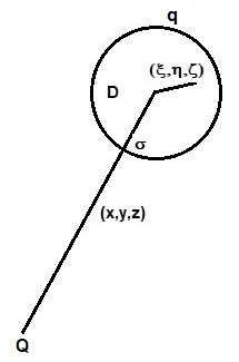
Let $\sigma$ be the radius of the little solid sphere, $(\xi,\eta,\zeta)$ its
local (Cartesian) coordinates and $\rho,\theta,\phi$ the spherical
coordinates equivalent of the latter. Then the test charge is modeled as:
$$
S(\xi,\eta,\zeta) = \left\{ \begin{array}{ll}
D & \mbox{for} \quad \xi^2+\eta^2+\zeta^2 < \sigma^2 \\
0 & \mbox{for} \quad \xi^2+\eta^2+\zeta^2 > \sigma^2 \end{array} \right.
\quad \mbox{or} \quad S(\rho) = \left\{ \begin{array}{ll}
D & \mbox{for} \quad \rho < \sigma \\
0 & \mbox{for} \quad \rho > \sigma \end{array} \right.
$$
Where $D$ is the (uniform) charge density of the solid sphere, which can be expressed in its
charge $q$ and its size $\sigma$:
$$
D \iiint S(\xi,\eta,\zeta) \, d\xi\, d\eta\, d\zeta = D \frac{4}{3}\pi \sigma^3 = q
\quad \Longleftrightarrow \quad D = q / \left(\frac{4}{3}\pi \sigma^3\right)
$$
The Coulomb field $F$ of the point charge $Q$ to be measured is given by:
$$
F(r) = \frac{q\cdot Q}{4\pi\epsilon_0\,r^2} = G\frac{q\cdot Q}{x^2 + y^2 + z^2}
$$
Where the constant $G$ - not the gravitational constant here - is conventiently defined by:
$$
G = \frac{1}{4\pi\epsilon_0}
$$
Now let $\vec{r}=(x,y,z)$ be the vector pointing
to the center of the solid test sphere with our point charge $Q$ as the origin. The force at
the test charge as a whole is then calculated as follows:
$$
\overline{F}(x,y,z) = G\cdot Q\cdot \iiint S(\xi,\eta,\zeta)
\frac{D\,d\xi\, d\eta\, d\zeta}{(x+\xi)^2 + (y+\eta)^2 + (z+\zeta)^2}
$$
Introducing spherical coordinates:
$$
\left\{ \begin{array}{l}
\xi = \rho \sin(\theta) \cos(\phi) \\
\eta = \rho \sin(\theta) \sin(\phi) \\
\zeta = \rho \cos(\theta) \end{array} \right.
\qquad \mbox{where} \quad 0 \le \theta \le \pi \quad \mbox{and} \quad 0 \le \phi \le 2\pi
$$
Because of the expected spherical symmetry of the problem, we only consider
a ray in $z$ direction, which means that $x = 0$ , $y = 0$ and $z = r$ .
The integral then becomes, after some suitable rearrangement:
$$
\overline{F}(r) = G\cdot Q\cdot q / \left(\frac{4}{3}\pi \sigma^3\right)
\int_0^{2\pi} d\phi \int_0^\sigma d\rho
\int_0^\pi \frac{\rho^2 \sin(\theta) \, d\theta}
{\rho^2 \sin^2(\theta) + \left[r + \rho \cos(\theta)\right]^2}
$$
Let's proceed with an abbreviation for the constant factor:
$$
C = G\cdot Q\cdot q / \left(\frac{4}{3}\pi \sigma^3\right)
$$
Then:
$$
\overline{F}(r) = -2\pi\,C
\int_0^\sigma d\rho \int_0^\pi \frac{\rho^2 \left[-\sin(\theta)\right] \, d\theta}
{\rho^2 + r^2 + 2\, r\rho \cos(\theta)}
$$ $$
= -2\pi\,C
\int_0^\sigma d\rho \frac{\rho}{2 r} \int_{\theta=0}^{\theta=\pi}
\frac{d\left[\rho^2 + r^2 + 2\, r\rho\cos(\theta)\right]}
{\rho^2 + r^2 + 2\, r\rho \cos(\theta)}
$$ $$
= -C\, \frac{2\pi}{2\, r}
\int_0^\sigma \rho \, d\rho
\left[ \ln\left(\rho^2 + r^2 + 2\, r\rho\cos(\theta)\right)
\right]_{\theta=0}^{\theta=\pi}
$$ $$
= + C\, \frac{2\pi}{2\, r}
\int_0^\sigma \left\{ \ln\left[(\rho + r)^2\right]
- \ln\left[(\rho - r)^2\right] \right\} \rho \, d\rho
$$
Substitution of $x = \rho/\sigma$ and $s = r/\sigma$ gives:
$$
\overline{F}(r) = C\, \frac{\pi\,\sigma^2}{r} \, \int_0^1
\left\{ \ln\left[(x + s)^2\right] - \ln\left[(x - s)^2\right] \right\}
x \, dx
$$
Divide and conquer one:
$$
\int \ln(x+s)^2 x \, dx =
$$ $$
\int \ln(x+s)^2 (x+s) \, d(x+s)
- s \int 2\, \ln|x+s| \, d(x+s) =
$$ $$
\frac{1}{2} (x+s)^2 \ln(x+s)^2 - \frac{1}{2}(x+s)^2
- 2 \, s \left[ (x+s)\ln|x+s| - (x+s) \right] =
$$ $$
(x^2 + 2 x s + s^2) \ln|x+s| - x^2/2 - x s - s^2/2
$$ $$
+ (- 2 x s - 2 s^2) \ln|x+s| + 2 x s + 2 s^2 =
$$ $$
(x^2 - s^2) \ln|x+s| - x^2/2 + x s + 3 s^2/2
$$
Divide and conquer two:
$$
\int \ln(x-s)^2 x \, dx =
$$ $$
\int \ln(x-s)^2 (x-s) \, d(x-s)
+ s \int 2\, \ln|x-s| \, d(x-s) =
$$ $$
\frac{1}{2} (x-s)^2 \ln(x-s)^2 - \frac{1}{2} (x-s)^2
+ 2 \, s \left[ (x-s)\ln|x-s| - (x-s) \right] =
$$ $$
(x^2 - 2 x s + s^2) \ln|x-s| - x^2/2 + x s - s^2/2
$$ $$
+ (2 x s - 2 s^2) \ln|x-s| - 2 x s + 2 s^2 =
$$ $$
(x^2 - s^2) \ln|x-s| - x^2/2 - x s + 3 s^2/2
$$
One and two must be substracted. And integrated from $0$ to $1$.
$$
\int_0^1 \left[ \ln(x+s)^2 - \ln(x-s)^2 \right] x \, dx =
$$ $$
\left[ (x^2 - s^2) \ln|x+s| - x^2/2 + x s + 3 s^2/2 \right]_{x=0}^{x=1} -
$$ $$
\left[ (x^2 - s^2) \ln|x-s| - x^2/2 - x s + 3 s^2/2 \right]_{x=0}^{x=1} =
$$ $$
\left[ (x^2 - s^2) \ln \left| \frac{x+s}{x-s} \right| + 2\, x s
\right]_{x=0}^{x=1} =
(1 - s^2) \ln \left| \frac{1+s}{1-s} \right| + 2\, s
$$
Consequently, the Coulomb field as felt by the test charge is:
$$
\overline{F}(r) = C\, \frac{\pi\,\sigma^2}{r} \,
\left\{ \left[1 - \left(\frac{r}{\sigma}\right)^2\right]
\ln \left| \frac{1+r/\sigma}{1-r/\sigma} \right| + 2\, \frac{r}{\sigma} \right\}
$$
There are a few singularities involved here. The first one is at $r=0$ , which
is easiest to calculate if we start from the basics all over.
$$
\overline{F}(0,0,0) = G\cdot Q \cdot \iiint S(\xi,\eta,\zeta)
\frac{d\xi\, d\eta\, d\zeta}{\xi^2 + \eta^2 + \zeta^2} \quad \Longleftrightarrow \quad
$$ $$
\overline{F}(0) = G\cdot Q \cdot q / \left(\frac{4}{3}\pi \sigma^3\right)
\int_0^\sigma \frac{4\pi\rho^2\, d\rho}{\rho^2} =
C\, 4\pi\, \sigma = \frac{3\,G Q q}{\sigma^2}
$$
The next singularity is where the denominator $(1-r/\sigma) $ in the logarithm for
$r=\sigma$ , or $(1-s)$ for $s=1$ , becomes zero.
$$
\lim_{s\rightarrow 1}
\left\{ (1 - s^2) \ln \left| \frac{1+s}{1-s} \right| + 2\, s \right\} =
$$ $$
\lim_{s\rightarrow 1}
\left\{ (1+s)(1-s)\ln|1+s| - (1+s)\left[ (1-s)\ln|1-s| \right]
+ 2\, s \right\} = 2
$$
Because $\lim_{x\rightarrow 0} x\ln(x) = 0$ with $x = (1-s)$ .
$$
\quad \Longrightarrow \quad
\overline{F}(\sigma) = C\, \frac{\pi\,\sigma^2}{\sigma}\, 2 = C\, 2\pi\, \sigma
= \frac{1}{2} \overline{F}(0) = \frac{3\,G Q q}{2\,\sigma^2} = \frac{3}{2} F(\sigma)
$$
We could have done it by hand, but with MAPLE it goes faster:
> simplify(diff((1-s^2)*ln((1+s)/(1-s))+2*s,s));
$$
-2 s \ln\left|\frac{1+s}{1-s}\right| + 4
$$
From this we see that for $s=1$ i.e. $r=\sigma$ the function $\overline{F}(r)$ has
a slope that is negative and infinitely large: $\overline{F'}(\sigma) = -\infty$ .
The Coulomb force as felt by the test charge can also be written as follows:
$$
\overline{F}(r) = C\, \frac{\pi\,\sigma^2}{r} \frac{r^2}{\sigma^2} \left\{
\left[\left(\frac{\sigma}{r}\right)^2 - 1\right]
\ln \left| \frac{\sigma/r+1}{\sigma/r-1} \right| + 2\, \frac{\sigma}{r} \right\}
$$
And with help of the variable $x = \sigma/r$ , which is small for $r \gg \sigma$ :
$$
= \frac{3\, G Q q }{4\, \sigma^2 x} \left\{
(x^2 - 1) \ln\left|\frac{x+1}{x-1}\right| + 2\, x \right\}
$$
We could have done it by hand, but with MAPLE it goes much faster:
> series(3/4/(\sigma^2*x)*((x^2-1)*ln((1+x)/(1-x))+2*x),x,7);
$$
\frac{1}{\sigma^2} x^2 + \frac{1}{5 \sigma^2} x^4 + \frac{3}{35 \sigma^2} x^6 + O(x^8)
\approx \frac{1}{\sigma^2} \left( \frac{\sigma}{r} \right)^2 = \frac{1}{r^2}
$$
Thus the standard Coulomb law (red) is valid for small values of $x$ , that is
for large values of $r$ , that is for $r \gg\sigma$ . The law as actually observed within
this model is depicted in black; yellow line at position $r = \sigma$ . See picture:
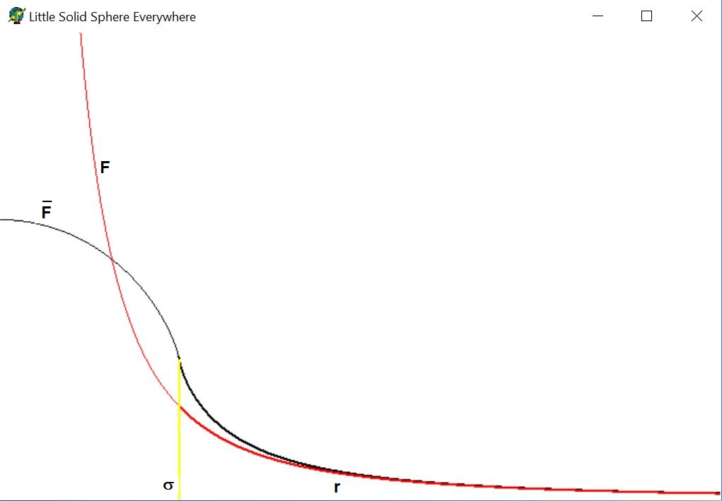
Remember that $r$ is the distance of the center of the test charge $q$ to the point charge $Q$.
Thus for $r < \sigma$ the point charge would be penetrating the test charge, which means that the
singularity would be inside the test charge. With other words: it is possible to measure the singularity
with our test charge. These are the thinner lines in that region. While this may seem physically improbable,
we shall assume that it is so.
The reason is that we want to calculate the Self Energy $U$ of the electron, as defined
by the formula ($V$ = space volume). According to classical electrodynamics, the outcome is catastrophical:
$$
E = \frac{Q}{4 \pi \epsilon_0 r^2} \quad \Longrightarrow \\
U = \int_0^\infty\frac{1}{2}\epsilon_0 \left(\frac{Q}{4\pi\epsilon_0 r^2}
\right)^2 4 \pi r^2 dr \ = \\
\frac{Q^2}{8 \pi \epsilon_0} \int_0^\infty \frac{dr}{r^2} = \infty
$$
So let's try instead the "measured" electrical force:
$$
U = \iiint \frac{1}{2} \epsilon_0 \overline{E}^{\,2} \, dV =
\int_0^\infty \frac{1}{2} \epsilon_0 \overline{E}^{\,2}(r)\, 4\pi r^2 \, dr
$$
What we have found is an expression for the renormalized electric force $\overline{F}$.
The electric field $\overline{E}$ is derived from it by dividing with the test charge $q$:
$$
\overline{E}(r) = \frac{C}{q}\,\frac{\pi\,\sigma^2}{r} \frac{r^2}{\sigma^2} \left\{
\left[\left(\frac{\sigma}{r}\right)^2 - 1\right]
\ln \left| \frac{\sigma/r+1}{\sigma/r-1} \right| + 2\, \frac{\sigma}{r} \right\}
$$
Where:
$$
C = G\cdot Q\cdot q / \left(\frac{4}{3}\pi \sigma^3\right) \quad ; \quad
G =\frac{1}{4\pi\epsilon_0}
$$
Let $x = r/\sigma$ in:
$$
\overline{E}(r) = \frac{Q}{4\pi\epsilon_0} \frac{3}{4 \sigma^2 r/\sigma} \,
\left\{ \left[1 - \left(\frac{r}{\sigma}\right)^2\right]
\ln \left| \frac{1+r/\sigma}{1-r/\sigma} \right| + 2\, \frac{r}{\sigma} \right\} =
$$ $$
\frac{Q}{4\pi\epsilon_0} \frac{3}{4 \sigma^2 x} \,
\left\{(1 - x^2) \ln \left| \frac{1+x}{1-x} \right| + 2\, x \right\} \quad \Longrightarrow \quad
$$ $$
U = \frac{Q^2}{8\pi\epsilon_0 \sigma} \left(\frac{3}{4}\right)^2 \, \int_0^\infty
\left\{(1 - x^2) \ln\left| \frac{1+x}{1-x} \right| + 2\, x \right\}^2 \, dx
$$
We could not have done this by hand, so let's see what MAPLE says about
it:
> f(x) := ((1-x^2)*ln(abs((1+x)/(1-x))+2*x)^2;
> int(expand(f(x)),x=0..infinity);
And the outcome is truly wonderful ..
$$
\frac{8 \pi^2}{15} \qquad \qquad \mbox{YES !!}
$$
Hence the Self Energy of the Electron is, according to this model:
$$
U = \frac{Q^2}{8\pi\epsilon_0 \sigma}\left(\frac{3}{4}\right)^2\frac{8 \pi^2}{15}
= \frac{3\,\pi^2}{20} \frac{Q^2}{4\pi\epsilon_0 \sigma} \\
U = m\,c^2 \quad \Longrightarrow \quad \sigma = \frac{3\,\pi^2}{20}\frac{1}{4\pi\epsilon_0}\frac{Q^2}{m\,c^2}
$$
The Classical electron radius
is defined (using our notation) by:
$$
a = \frac{1}{4\pi\epsilon_0} \frac{Q^2}{m\,c^2} \approx 2.8179403227(19)\times 10^{-15}\,m
$$
Therefore the radius of the electron as measured by our little green uniformly charged solid sphere is
roughly one and a half times the classical electron radius $a$ :
$$
\sigma = \frac{3\,\pi^2}{20} \, a
$$
Instead of the uniformly charged solid sphere we could have adopted some other mathematical model for the measuring device
(for example a Gaussian distribution has been tried in the 1995 version of the book).
This would have resulted in a factor whch is somewhat different, but not very much deviant from our present value $\approx 3/2$ .
It might thus be concluded that the "true" electron radius is somewhat unclear indeed, but anyway not significantly different
from the classical electron radius. Quod Erat Demonstrandum (QED :-)